Extract Event Statistics in Hydrologic Time Series.
hydroEvents
Events from individual hydrologic time series are extracted, and events from multiple time series can be matched to each other.
This code can be downloaded from CRAN: https://cran.r-project.org/package=hydroEvents
A detailed description of each function, usage, and suggested parameters is provided in the following: Wasko, C., Guo, D., 2022. Understanding event runoff coefficient variability across Australia using the hydroEvents R package. Hydrol. Process. 36, e14563. https://doi.org/10.1002/hyp.14563
If using this code a citation to the above manuscript would be greatly appreciated.
Example 1
Aim: Calculate baseflow and baseflow index
This code reproduces Figure 5 in Wasko and Guo (2022).
library(hydroEvents)
bf.A.925 = baseflowA(dataBassRiver, alpha = 0.925)$bf
bf.A.980 = baseflowA(dataBassRiver, alpha = 0.980)$bf

bf.B.925 = baseflowB(dataBassRiver, alpha = 0.925)$bf
bf.B.980 = baseflowB(dataBassRiver, alpha = 0.980)$bf

bfi.A.925 = sum(bf.A.925)/sum(dataBassRiver) # 0.22
bfi.A.980 = sum(bf.A.980)/sum(dataBassRiver) # 0.09
bfi.B.925 = sum(bf.B.925)/sum(dataBassRiver) # 0.39
bfi.B.980 = sum(bf.B.980)/sum(dataBassRiver) # 0.20

plot(dataBassRiver, type = "l", col = "#377EB8", lwd = 2, mgp = c(2, 0.6, 0), ylab = "Flow (ML/day)", xlab = "Index", xlim = c(0, 70))
lines(bf.A.925, lty = 2)
lines(bf.A.980, lty = 3)
lines(bf.B.925, lty = 1)
lines(bf.B.980, lty = 4)
legend("topright", lty = c(2, 3, 1, 4), col = c("black", "black", "black", "black"), cex = 0.8, bty = "n",
       legend = c(paste0("BFI(A, 0.925) = ", format(round(bfi.A.925, 2), nsmall = 2)),
                  paste0("BFI(A, 0.980) = ", format(round(bfi.A.980, 2), nsmall = 2)),
                  paste0("BFI(B, 0.925) = ", format(round(bfi.B.925, 2), nsmall = 2)),
                  paste0("BFI(B, 0.980) = ", format(round(bfi.B.980, 2), nsmall = 2))))

Example 2
Aim: Extract precipitation events
events = eventPOT(dataLoch, threshold = 1, min.diff = 2)
plotEvents(dataLoch, dates = NULL, events = events, type = "hyet", ylab = "Rainfall [mm]", main = "Rainfall Events (threshold = 1, min.diff = 2)")

Example 3
Aim: Extract flow events (and demonstrate the different methods available)
This code reproduces Figure 6 in Wasko and Guo (2022).
library(hydroEvents)
bf = baseflowB(dataBassRiver)
Max_res = eventMaxima(dataBassRiver-bf$bf, delta.y = -0.75, delta.x = 1, threshold = 0)
Min_res = eventMinima(dataBassRiver-bf$bf, delta.y = 100, delta.x = 3, threshold = 0)
PoT_res = eventPOT(dataBassRiver-bf$bf, threshold = 0, min.diff = 1)
BFI_res = eventBaseflow(dataBassRiver, BFI_Th = 0.5, min.length = 1)

par(mfrow = c(2, 2), mar = c(3, 2.7, 2, 1))
plotEvents(data = dataBassRiver, events = PoT_res, ymax = 1160, xlab = "Index", ylab = "Flow (ML/day)", colpnt = "#E41A1C", colline = "#377EB8", main = "eventPOT")
lines(1:length(bf$bf), bf$bf, lty = 2)
plotEvents(data = dataBassRiver, events = Max_res, ymax = 1160, xlab = "Index", ylab = "Flow (ML/day)", colpnt = "#E41A1C", colline = "#377EB8", main = "eventMaxima")
lines(1:length(bf$bf), bf$bf, lty = 2)
plotEvents(data = dataBassRiver, events = Min_res, ymax = 1160, xlab = "Index", ylab = "Flow (ML/day)", colpnt = "#E41A1C", colline = "#377EB8", main = "eventMinima")
lines(1:length(bf$bf), bf$bf, lty = 2)
plotEvents(data = dataBassRiver, events = BFI_res, ymax = 1160, xlab = "Index", ylab = "Flow (ML/day)", colpnt = "#E41A1C", colline = "#377EB8", main = "eventBaseflow")
lines(1:length(bf$bf), bf$bf, lty = 2)

Example 4
Aim: Identify rising and falling limbs
library(hydroEvents)
qdata = WQ_Q$qdata[[1]]
BF_res = eventBaseflow(qdata$Q_cumecs)
limbs(data = qdata$Q_cumecs, dates = NULL, events = BF_res, main = "with 'eventBaseflow'")

Example 5
Aim: Calculate CQ (concentration-discharge) relationships
library(hydroEvents)
# Identify flow events
qdata = WQ_Q$qdata[[1]]
BF_res = eventBaseflow(qdata$Q_cumecs)
MAX_res = eventMaxima(qdata$Q_cumecs, delta.y = 0.5, threshold = 0.5)

# Aggregate water quality data to daily time step
wqdata=WQ_Q$wqdata[[1]]
wqdata = data.frame(time=wqdata$time,wq=as.vector(wqdata$WQ))

wqdaily = rep(NA,length(unique(substr(wqdata$time,1,10))))
for (i in 1:length(unique(substr(wqdata$time,1,10)))) {
  wqdaily[i] = mean(wqdata$wq[which(substr(wqdata$time,1,10)==
                                      unique(substr(wqdata$time,1,10))[i])])
}
wqdailydata = data.frame(time=as.Date(strptime(unique(substr(wqdata$time,1,10)),"%d/%m/%Y")),wq=wqdaily)

# A function to plot the CQ relationship by event period
CQ_event = function(C,Q,events,methodname) {
  QinWQ = which(Q$time%in%C$time)

  risfal_res = limbs(data=as.vector(Q$Q_cumecs),events=events,main = paste("Events identified -",methodname))

  allRL_ind = unlist(apply(risfal_res,1,function(x){x[6]:x[7]}))
  allFL_ind = unlist(apply(risfal_res,1,function(x){x[8]:x[9]}))

  RL_ind = which(allRL_ind%in%QinWQ)
  FL_ind = which(allFL_ind%in%QinWQ)

  allEV_ind = unlist(apply(risfal_res,1,function(x){x[1]:x[2]}))
  allBF_ind = as.vector(1:length(as.vector(Q$Q_cumecs)))[-allEV_ind]
  EV_ind = which(allEV_ind%in%QinWQ)
  BF_ind = which(allBF_ind%in%QinWQ)

  RL_indwq = which(QinWQ%in%allRL_ind[RL_ind])
  FL_indwq = which(QinWQ%in%allFL_ind[FL_ind])
  BF_indwq = which(QinWQ%in%allBF_ind[BF_ind])
  EV_indwq = which(QinWQ%in%allEV_ind[EV_ind])

  plot(C$wq~Q$Q_cumecs[QinWQ],xlab="Q (mm/d)",ylab="C (mg/L)",main = paste("C-Q relationship -",methodname),pch=20)
  points(C$wq[RL_indwq]~Q$Q_cumecs[allRL_ind[RL_ind]],col="blue",pch=20)
  points(C$wq[FL_indwq]~Q$Q_cumecs[allFL_ind[FL_ind]],col="red",pch=20)
  points(C$wq[BF_indwq]~Q$Q_cumecs[allBF_ind[BF_ind]],col="grey",pch=20)

  legend("topright",
         legend=c("rising limb","falling limb","baseflow"),
         pch=20,col=c("blue","red","grey"))

  CQ = cbind(C$wq,Q$Q_cumecs[QinWQ])
  res = list(event=EV_indwq,base=BF_indwq,rising=RL_indwq,falling=FL_indwq,
             eventCQ=CQ[EV_indwq,],baseCQ=CQ[BF_indwq,],
             risingCQ=CQ[RL_indwq,],fallingCQ=CQ[FL_indwq,])
}

# Final plot of CQ comparison from two event approaches
par(mfcol=c(2,2))
par(mar=c(2,2,2,2))
CQ_event(wqdailydata,qdata, BF_res, methodname="eventBaseflow")
CQ_event(wqdailydata,qdata, MAX_res, methodname="eventMaxima")
Example 6
Aim: Demonstrate matching rainfall to runoff
library(hydroEvents)
# Prepare data
srt = as.Date("2015-02-05")
end = as.Date("2015-04-01")
dat = dataCatchment$`105105A`[which(dataCatchment$`105105A`$Date >= srt & dataCatchment$`105105A`$Date <= end),]

# Extract events
events.P = eventPOT(dat$Precip_mm, threshold = 1, min.diff = 1)
events.Q = eventMaxima(dat$Flow_ML, delta.y = 2, delta.x = 1, thresh = 70)

par(mfrow = c(2, 1), mar = c(3, 2.7, 2, 1))
plotEvents(dat$Precip_mm, dates = dat$Date, events = events.P, type = "hyet", colline = "#377EB8", colpnt = "#E41A1C",ylab = "Rainfall (mm)", xlab = 2015, main = "")
plotEvents(dat$Flow_ML,   dates = dat$Date, events = events.Q, type = "lineover", colpnt = "#E41A1C", colline = "#377EB8", ylab = "Flow (ML/day)", xlab = 2015, main = "")

The following code reproduces Figure 7 in Wasko and Guo (2022).
# Match events
library(RColorBrewer)
matched.1 = pairEvents(events.P, events.Q, lag = 5,  type = 1)
matched.2 = pairEvents(events.P, events.Q, lag = 5,  type = 2)
matched.3 = pairEvents(events.P, events.Q, lag = 3,  type = 3)
matched.4 = pairEvents(events.P, events.Q, lag = 7, type = 4)
matched.5 = pairEvents(events.P, events.Q, lag = 5, type = 5)

par(mfrow = c(3, 2), mar = c(1.7, 3, 2.1, 3))
plotPairs(data.1 = dat$Precip_mm, data.2 = dat$Flow_ML, events = matched.1, date = dat$Date, col = brewer.pal(nrow(events.P), "Set3"), main = "Type 1", ylab.1 = "Rainfall (mm)", ylab.2 = "Flow (ML/day)", cex.2 = 2/3)
plotPairs(data.1 = dat$Precip_mm, data.2 = dat$Flow_ML, events = matched.2, date = dat$Date, col = brewer.pal(nrow(events.P), "Set3"), main = "Type 2", ylab.1 = "Rainfall (mm)", ylab.2 = "Flow (ML/day)", cex.2 = 2/3)
plotPairs(data.1 = dat$Precip_mm, data.2 = dat$Flow_ML, events = matched.3, date = dat$Date, col = brewer.pal(nrow(events.P), "Set3"), main = "Type 3", ylab.2 = "Rainfall (mm)", ylab.1 = "Flow (ML/day)", cex.2 = 2/3)
plotPairs(data.1 = dat$Precip_mm, data.2 = dat$Flow_ML, events = matched.4, date = dat$Date, col = brewer.pal(nrow(events.P), "Set3"), main = "Type 4", ylab.2 = "Rainfall (mm)", ylab.1 = "Flow (ML/day)", cex.2 = 2/3)
plotPairs(data.1 = dat$Precip_mm, data.2 = dat$Flow_ML, events = matched.5, date = dat$Date, col = brewer.pal(nrow(events.P), "Set3"), main = "Type 5", ylab.1 = "Rainfall (mm)", ylab.2 = "Flow (ML/day)", cex.2 = 2/3)

Example 7
Aim: Demonstrate matching of rainfall and water level surge (residuals)
library(hydroEvents)

# Hourly rainfall (P) and water level surge (WL) at Burnie, Tasmania (Pluvio 91009; Tide gauge: IDO71005)
Psel  = data_P_WL$Psel
WLsel = data_P_WL$WLsel

# Find events in P and WL data
# Rain over 4mm is considered an event; events over 3 hrs apart are considered as separate
events.P = eventPOT(Psel, threshold = 4, min.diff = 3)

# WL surge residual over 0.05m is considered an event; events over 3 hrs apart are considered as separate
events.Q1 = eventMaxima(WLsel, delta.y = 0.05, delta.x = 3, thresh = 0.05)

# Plot events
plotEvents(data = Psel, events = events.P, main = "Hourly precipitation (mm)", type = "hyet")
plotEvents(data = WLsel, events = events.Q1, main = "Hourly water level surge (m)", type = "lineover")

# Pairing events - use type = 5 to search both ways for the pairing
# Try two different values for the lag (search radius)
matched.1 = pairEvents(events.P, events.Q1, lag = 12, type = 5)
matched.2 = pairEvents(events.P, events.Q1, lag = 24, type = 5)

plotPairs(data.1 = Psel, data.2 = WLsel, events = matched.1, type = "hyet", color.list=rainbow(nrow(matched.1)))
plotPairs(data.1 = Psel, data.2 = WLsel, events = matched.2, type = "hyet", color.list=rainbow(nrow(matched.2)))

Example 8
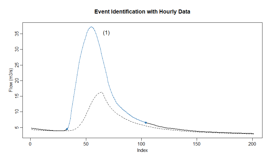
Aim: Demonstrate event identification with hourly streamflow data
library(hydroEvents)
library(stats)
# Prepare data
data(hourlyQ)

# smoothing for hourly data to remove local fluctuation
flow = hourlyQ$q
n = length(flow)
flow.smoothed = filter(flow, c(0.1, 0.2, 0.4, 0.2, 0.1))[3:(n-2)]

# baseflow filtering and event identification with eventMaxima
bf = baseflowA(flow.smoothed, alpha = 0.925)
events = eventMaxima(flow.smoothed-bf$bf, -0.75, 12, threshold = 1)
idx = 63800
events$srt = events$srt - idx
events$end = events$end - idx
plotEvents(data = flow[3:(n-2)][idx:(idx+200)], events = events[120,], type = "lineover", xlab = "Index", ylab = "Flow (m3/s)", colpnt = "#E41A1C", colline = "#377EB8", main = "Event Identification with Hourly Data")
lines(1:201, bf$bf[idx:(idx+200)], lty = 2)

Example 9
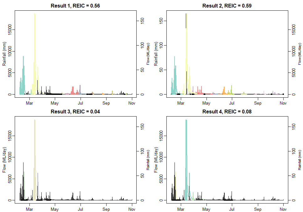
Aim: Demonstrate the calculation of the Robust Event Identification Criteria (REIC), following Mohammadpour Khoie, et al. (2025): https://doi.org/10.1016/j.envsoft.2025.106521. Calculation of the REIC value for a set of rainfall-runoff events given rainfall and runoff time series and events
library(RColorBrewer)
dat = dataCatchment$`105105A`
srt = as.Date("2015-02-05")
end = as.Date("2015-11-01")
dat = dataCatchment$`105105A`[which(dataCatchment$`105105A`$Date >= srt & dataCatchment$`105105A`$Date <= end),]


events.P = eventPOT(dat$Precip_mm, threshold = 1, min.diff = 1)
QF <- dat$Flow_ML-baseflowA(dat$Flow_ML, alpha = 0.925, passes = 3)$bf
events.Qbest1 = eventMinima(QF, delta.y = 14.24, delta.x = 1, thresh = 6.58)
matched.best1 = PostCorrection(pairEvents(events.P, events.Qbest1, lag = 6,  type = 3))

events.Qbest2 = eventMinima(QF, delta.y = 21.37, delta.x = 5, thresh = 2.42)
matched.best2 = PostCorrection(pairEvents(events.P, events.Qbest1, lag = 7,  type = 5))

events.Qworst1 = eventMaxima(QF, delta.y = -0.861, delta.x = 1, thresh = 127.1)
matched.worst1 = PostCorrection(pairEvents(events.P, events.Qworst1, lag = 1,  type = 4))

events.Qworst2 = eventMaxima(QF, delta.y = -0.825, delta.x = 9, thresh = 39.26)
matched.worst2 = PostCorrection(pairEvents(events.P, events.Qworst2, lag = 1,  type = 4))

REIC.b1 <- round(calcREIC(dat$Precip_mm, dat$Flow_ML, matched.best1, n_rainfall = nrow(events.P), area = 297),2) # see manual 'dataCatchment'
REIC.b2 <- round(calcREIC(dat$Precip_mm, dat$Flow_ML, matched.best2, n_rainfall = nrow(events.P), area = 297),2) # see manual 'dataCatchment'

REIC.w1 <- round(calcREIC(dat$Precip_mm, dat$Flow_ML, matched.worst1, n_rainfall = nrow(events.P), area = 297),2) # see manual 'dataCatchment'
REIC.w2 <- round(calcREIC(dat$Precip_mm, dat$Flow_ML, matched.worst2, n_rainfall = nrow(events.P), area = 297),2) # see manual 'dataCatchment'

par(mfrow = c(2, 2), mar = c(1.7, 3, 2.1, 3))
plotPairs(data.1 = dat$Precip_mm, data.2 = dat$Flow_ML, events = matched.best1, date = dat$Date, col = colorRampPalette(brewer.pal(12, "Set3"))(nrow(events.P)),
          main = paste("Result 1, REIC =",REIC.b1), ylab.1 = "Rainfall (mm)", ylab.2 = "Flow (ML/day)", cex.2 = 2/3)
plotPairs(data.1 = dat$Precip_mm, data.2 = dat$Flow_ML, events = matched.best2, date = dat$Date, col = colorRampPalette(brewer.pal(12, "Set3"))(nrow(events.P)),
          main = paste("Result 2, REIC =",REIC.b2), ylab.1 = "Rainfall (mm)", ylab.2 = "Flow (ML/day)", cex.2 = 2/3)
plotPairs(data.1 = dat$Precip_mm, data.2 = dat$Flow_ML, events = matched.worst1, date = dat$Date, col = colorRampPalette(brewer.pal(12, "Set3"))(nrow(events.P)),
          main = paste("Result 3, REIC =",REIC.w1), ylab.2 = "Rainfall (mm)", ylab.1 = "Flow (ML/day)", cex.2 = 2/3)
plotPairs(data.1 = dat$Precip_mm, data.2 = dat$Flow_ML, events = matched.worst2, date = dat$Date, col = colorRampPalette(brewer.pal(12, "Set3"))(nrow(events.P)),
          main = paste("Result 4, REIC =",REIC.w2), ylab.2 = "Rainfall (mm)", ylab.1 = "Flow (ML/day)", cex.2 = 2/3)
