K Nearest Neighbor Forecasting with a Tailored Similarity Metric.

knnwtsim

The goal of knnwtsim is to provide a package to share and implement a forecasting methodology using k nearest neighbors (KNN) primarily for situations where the response series of interest can be predicted by a combination of its’ own recent realizations, its own periodic patterns, and by the values of one or multiple exogenous predictors.

The functions of this package are focused primarily into two components. The first being calculation of a similarity measure which takes into account all three factors listed above (S_w), and can weight the degree to which each component contributed to the overall similarity. The second being the usage of this measure to identify neighbors and perform KNN regression. For a more formal discussion of the methodology used and the key user facing functions in knnwtsim please see Trupiano (2021) \<arXiv:2112.06266v1>.

Formulation

Weighted Similarity Measure S_w

The Similarity measure I have formulated for incorporating the three factors listed above is:

S_w = alpha * S_t + beta * S_p + gamma * S_x

Where S_t is the metric used to calculate the similarity matrix generated by StMatrixCalc to measure similarity in terms of pure recency between all observations. alpha is the weight between 0-1 assigned to this matrix in the calculation of S_w.

S_p is the metric used to calculate the similarity matrix generated by SpMatrixCalc to measure similarity in terms of where each observation falls along a periodic cycle relative to all others. beta is the weight between 0-1 assigned to this matrix in the calculation of S_w.

S_x is the metric used to calculate the similarity matrix generated by SxMatrixCalc to measure similarity between all observations in terms of the values of one or more exogenous predictors associated with a given observation. gamma is the weight between 0-1 assigned to this matrix in the calculation of S_w.

The function SwMatrixCalc calls each of the previous similarity matrix functions to generate the final matrix to use in knn.forecast.

The weights alpha, beta, and gamma are recommended to be set so that they sum to 1. In this case each element of final similarity matrix should also be between 0-1, with the diagonal elements being equal to 1.

Component Similarity Details

Initially S_t, S_p, and S_x are calculated as dissimilarities, D_t, D_p, and D_x. They are then transformed to similarities by the formula 1 / (D+1), where D is any dissimilarity measure. This also ensures each element of the similarity matrices fall in the range (0,1], with 1 representing the greatest similarity, and the values approaching 0 the least.

When StMatrixCalc generates the intermediate dissimilarity matrix using D_t, it calls the function TempAbsDissimilarity for each pairwise combination of the input vector. Which provided the time orders of two points y_i and y_j, where the time orders are i and j.Then TempAbsDissimilarity(i, j) will return the absolute difference between the two, i.e abs(i - j).

When SpMatrixCalc generates the intermediate dissimilarity matrix using D_p, it calls the function SeasonalAbsDissimilarity for each pairwise combination of the input vector. This function takes the values corresponding to the periods of two points in an overall periodic/seasonal cycle, and the total number of periods in a cycle. Where we have two points y_i and y_j with p_i and p_j representing the corresponding period of those points, and a total of p_max periods in a full periodic cycle. The value returned by SeasonalAbsDissimilarity(p_i, p_j, p_max) will be min(DirectDis, AroundDis) where DirectDis <- abs(p_i - p_j) and AroundDis <- abs(min(p_i, p_j) - 1) + abs(p_max - max(p_i, p_j)) + 1.

This formulation is based on the idea that generally the periods at the very end and very beginning of a cycle should be fairly similar. To clarify through an example, in a monthly cycle where 1 represents January and 12 represents December, these two months are generally more similar to each-other than either are to July at period 7. Continuing with this monthly example, if we have three points which occur in January, March, and November: p_i = 1, p_j = 3, p_k = 11 with p_max = 12. Then SeasonalAbsDissimilarity(p_i, p_j, p_max) = 2, SeasonalAbsDissimilarity(p_i, p_k, p_max) = 2, and SeasonalAbsDissimilarity(p_j, p_k, p_max) = 4.

Finally, SxMatrixCalc uses the stats::dist function to produce the intermediate dissimilarity matrix using D_x, for an input matrix or vector using the method indicated by the XdistMetric argument of SxMatrixCalc. Naturally, this limits D_x to the methods available in stats::dist.

KNN Forecasting

K nearest neighbors forecasting is implemented in this package through the function knn.forecast. Using a provided similarity matrix, which is not required to be calculated using S_w specifically, the function will perform K Nearest Neighbors regression on each point in a specified index f.index.in, returning the mean of the identified, k.in, neighbors in the response series y.in.

Mathematically the estimate for a given point y_t is formulated as the mean of the previous points in the series y_i identified to be in the neighborhood of y_t, K(y_t).

In the neighborhood K(y_t) will be the k observations of y_i with the highest similarity to y_t of all eligible members of the time series, meaning i < t. Currently in knn.forecast this eligibility constraint is enforced by only considering the rows of the similarity matrix at indices which are not present in f.index.in when selecting neighbors while performing KNN regression on each point in f.index.in, thus preventing the corresponding points in y.in at those indices from being selected as neighbors. Furthermore, rows and columns of Sim.Mat.in at indices greater than the maximum value of f.index.in will be removed.

Installation

You can install the most recent stable version from CRAN with

install.packages("knnwtsim")

You can install the development version of knnwtsim from GitHub with:

# install.packages("devtools")
devtools::install_github("mtrupiano1/knnwtsim")

Example with Known Similarity Matrix Weights and k

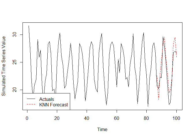
This is a basic example which shows a full forecasting workflow if the weights to use in the generation of S_w, and the hyperparameter k are known:

library(knnwtsim)
# Pull a series to forecast
data("simulation_master_list")
series.index <- 15
ex.series <- simulation_master_list[[series.index]]$series.lin.coef.chng.x

# Weights pre tuned by random search. In alpha, beta, gamma order
pre.tuned.wts <- c(0.2148058, 0.2899638, 0.4952303)
pre.tuned.k <- 5

df <- data.frame(ex.series)
# Generate vector of time orders
df$t <- c(1:nrow(df))

# Generate vector of periods
nperiods <- simulation_master_list[[series.index]]$seasonal.periods
df$p <- rep(1:nperiods, length.out = nrow(df))

# Pull corresponding exogenous predictor(s)
X <- as.matrix(simulation_master_list[[series.index]]$x.chng)
XdistMetric <- "euclidean"

# Number of points to set aside for validation
val.len <- ifelse(nperiods == 12, nperiods, nperiods * 2)

# Calculate the weighted similarity matrix using Sw
Sw.ex <- SwMatrixCalc( # For the recency similarity St
  t.in = df$t
  # For the periodic similarity Sp
  , p.in = df$p, nPeriods.in = nperiods
  # For the exogenous similarity Sx
  , X.in = X, XdistMetric.in = XdistMetric
  # Weights to be applied to each similarity
  , weights = pre.tuned.wts
)

# View the top corner of the weighted similarity matrix Sw
cat("\n Dimensions and Slice of S_w \n")
#> 
#>  Dimensions and Slice of S_w
print(dim(Sw.ex))
#> [1] 100 100
print(Sw.ex[1:5, 1:5])
#>           1         2         3         4         5
#> 1 0.9999999 0.5825337 0.4249690 0.4115130 0.5589633
#> 2 0.5825337 0.9999999 0.5989170 0.5690332 0.4841708
#> 3 0.4249690 0.5989170 0.9999999 0.6673498 0.4414853
#> 4 0.4115130 0.5690332 0.6673498 0.9999999 0.5582553
#> 5 0.5589633 0.4841708 0.4414853 0.5582553 0.9999999

# Index we want to forecast
val.index <- c((length(ex.series) - val.len + 1):length(ex.series))

# Generate the forecast
knn.frcst <- knn.forecast(
  Sim.Mat.in = Sw.ex,
  f.index.in = val.index,
  k.in = pre.tuned.k,
  y.in = ex.series
)

Example with Tuning of Similarity Matrix Weights

In most cases you will likely want to tune the hyperparameters used in the construction of S_w, and the number of nearest neighbors, k, to consider for any given point. There are many approaches that can be taken to accomplish this tuning, and many users may choose to implement their preferred approach. However, for those who want something pre-built I have included a simple tuning function with the package called knn.forecast.randomsearch.tuning. This function creates a randomly generated Grid of potential sets of hyperparameters k,alpha,beta,gamma and generates a forecast of length test.h on the last test.h points in the series. The best set of parameters are selected based on which row of the Grid led to the forecast with the lowest MAPE (Mean Absolute Percent Error) over the points in the forecast, and returned as the weight.opt and k.opt items of the list object returned by the function. Additionally, the ‘optimal’ similarity matrix to pass to knn.forecast is also returned as Sw.opt, as are the testing grid (Grid), best test MAPE (Test.MAPE.opt), and the full vector of test MAPE values (MAPE.all) corresponding to each row in Grid.

If you do not want to tune the hyperparameters on the entire series and prefer to leave some points for validation of the tuned result the val.holdout.len will remove that many points from the end of the series, and will perform the test forecasts on the test.h points at the end of the series after the validation observations are removed.

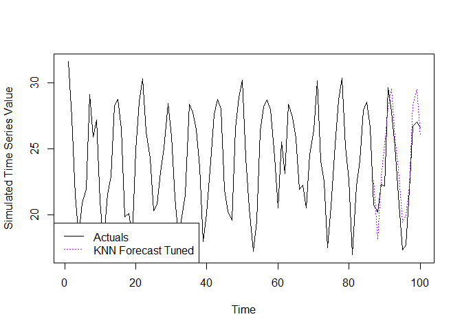
Using the example series from the previous section, we can reproduce the ‘pre-tuned’ weights from the previous section and generate a forecast using the included tuning function.

# Calculate component similarity matrices
St.ex <- StMatrixCalc(df$t)
Sp.ex <- SpMatrixCalc(df$p, nPeriods = nperiods)
Sx.ex <- SxMatrixCalc(X)

# Set seed for reproducibility
set.seed(10)
# Run tuning function
tuning.ex <- knn.forecast.randomsearch.tuning(
  grid.len = 10**4,
  y.in = ex.series,
  St.in = St.ex,
  Sp.in = Sp.ex,
  Sx.in = Sx.ex,
  test.h = val.len,
  max.k = NA,
  val.holdout.len = val.len
)


cat("\n Tuned Hyperparameters \n")
#> 
#>  Tuned Hyperparameters
cat("\n S_w Weights \n")
#> 
#>  S_w Weights
print(tuning.ex$weight.opt)
#> [1] 0.2148058 0.2899638 0.4952303
cat("\n k \n")
#> 
#>  k
print(tuning.ex$k.opt)
#> [1] 5

# Pull out tuned S_w and k
k.opt.ex <- tuning.ex$k.opt
Sw.opt.ex <- tuning.ex$Sw.opt

# Generate the forecast
knn.frcst.tuned <- knn.forecast(
  Sim.Mat.in = Sw.opt.ex,
  f.index.in = val.index,
  k.in = k.opt.ex,
  y.in = ex.series
)

Forecasting with Prediction Intervals

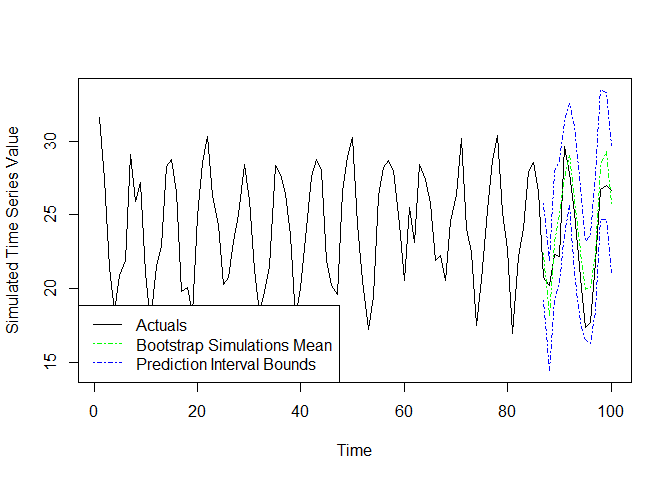
The methodology used to produce forecasts with prediction intervals in this package is based on the description of “Prediction intervals from bootstrapped residuals” from chapter 5.5 of Hyndman R, Athanasopoulos G (2021) https://otexts.com/fpp3/prediction-intervals.html#prediction-intervals-from-bootstrapped-residuals, modified as needed for use with KNN regression. The function knn.forecast.boot.intervals is used to implement this method. The algorithm employed starts by calculating a pool of forecast errors to later sample from. If there are n points prior to the first observation indicated in f.index.in then there will be n - k.in errors generated by one-step ahead forecasts starting with the point of the response series at the index k.in + 1. The first k.in points cannot be estimated because a minimum of k.in eligible neighbors would be needed. The optional burn.in argument can be used to increase the number of points from the start of the series that need to be available as neighbors before calculating errors for the pool. Next, B possible paths the series could take are simulated using the pool of errors. Each path is simulated by calling knn.forecast, estimating the first point in f.index.in, adding a sampled forecast error, then adding this value to the end of the series. This process is then repeated for the next point in f.index.in until all have been estimated. The final output interval estimates are calculated for each point in f.index.in by taking the appropriate percentiles of the corresponding simulations of that point. The output is returned as a list with the upper and lower prediction interval bounds based on the supplied confidence level, as well as the mean and median of the simulated points for each observation in the forecast index. All B simulations can be returned if desired using the optional return.simulations = TRUE argument. Below we have an example, where we generate an interval forecast at the 95% confidence level, and plot the results. Note that the mean forecast from this function may differ from the point forecast generated by knn.forecast. This difference is driven by the random sampling of residuals to generate the simulated paths, as well as the behavior of adding simulated points in a given path to the list of eligible neighbors when repeatably calling knn.forecast.

# Produce interval forecast list
interval.forecast <- knn.forecast.boot.intervals(
  Sim.Mat.in = Sw.opt.ex,
  f.index.in = val.index,
  y.in = ex.series,
  k.in = k.opt.ex
)

# Pull out desired components
lb <- interval.forecast$lb
ub <- interval.forecast$ub
mean.boot <- interval.forecast$mean