Fits a Collection of Curves to Single-Cohort Decomposition Data.

litterfitter

R package for fitting and testing alternative models for single cohort litter decomposition data

Installation

  #install.packages("remotes")
  remotes::install_github("cornwell-lab-unsw/litterfitter")
  
library(litterfitter)

Getting started

At the moment there is one key function which is fit_litter which can fit 6 different types of decomposition trajectories. Note that the fitted object is a litfit object

fit <- fit_litter(time=c(0,1,2,3,4,5,6),
                  mass.remaining =c(1,0.9,1.01,0.4,0.6,0.2,0.01),
                  model="weibull",
                  iters=500)

class(fit)

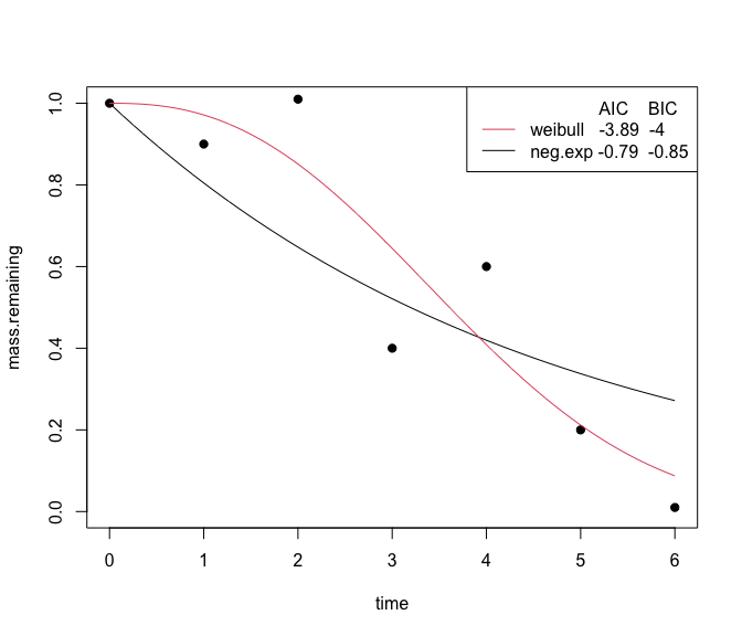
You can visually compare the fits of different non-linear equations with the plot_multiple_fits function:

plot_multiple_fits(time=c(0,1,2,3,4,5,6),
                   mass.remaining=c(1,0.9,1.01,0.4,0.6,0.2,0.01),
                   model=c("neg.exp","weibull"),
                   iters=500)

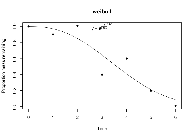
Calling plot on a litfit object will show you the data, the curve fit, and even the equation, with the estimated coefficients:

   plot(fit)

The summary of a litfit object will show you some of the summary statistics for the fit.

#> Summary of litFit object
#> Model type: weibull 
#> Number of observations:  7 
#> Parameter fits: 4.19 
#> Parameter fits: 2.47 
#> Time to 50% mass loss: 3.61 
#> Implied steady state litter mass: 3.71 in units of yearly input 
#> AIC:  -3.8883 
#> AICc:  -0.8883 
#> BIC:  -3.9965

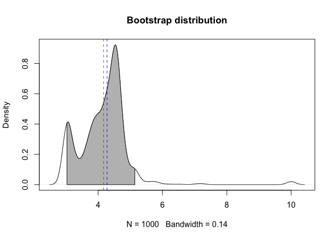
From the litfit object you can then see the uncertainty in the parameter estimate by bootstrapping.