Description
Cluster High Dimensional Categorical Datasets.
Description
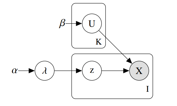
Scalable Bayesian clustering of categorical datasets. The package implements a hierarchical Dirichlet (Process) mixture of multinomial distributions. It is thus a probabilistic latent class model (LCM) and can be used to reduce the dimensionality of hierarchical data and cluster individuals into latent classes. It can automatically infer an appropriate number of latent classes or find k classes, as defined by the user. The model is based on a paper by Dunson and Xing (2009) <doi:10.1198/jasa.2009.tm08439>, but implements a scalable variational inference algorithm so that it is applicable to large datasets. It is described and tested in the accompanying paper by Ahlmann-Eltze and Yau (2018) <doi:10.1109/DSAA.2018.00068>.
README.md
mixdir
The goal of mixdir is to cluster high dimensional categorical datasets.
It can
- handle missing data
- infer a reasonable number of latent class (try
mixdir(select_latent=TRUE)) - cluster datasets with more than 70,000 observations and 60 features
- propagate uncertainty and produce a soft clustering
A detailed description of the algorithm and the features of the package can be found in the the accompanying paper. If you find the package useful please cite
C. Ahlmann-Eltze and C. Yau, "MixDir: Scalable Bayesian Clustering for High-Dimensional Categorical Data", 2018 IEEE 5th International Conference on Data Science and Advanced Analytics (DSAA), Turin, Italy, 2018, pp. 526-539.
Installation
install.packages("mixdir")

# Or to get the latest version from github
devtools::install_github("const-ae/mixdir")
Example
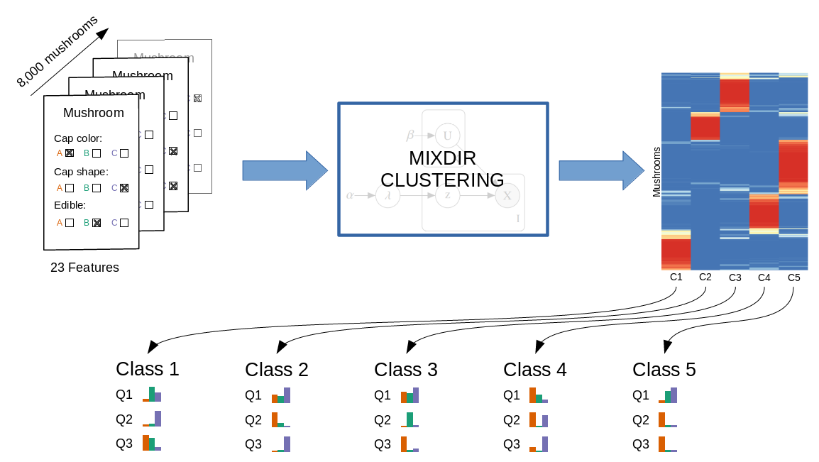
Clustering the mushroom data set.
# Loading the library and the data
library(mixdir)
set.seed(1)

data("mushroom")
# High dimensional dataset: 8124 mushroom and 23 different features
mushroom[1:10, 1:5]
#>    bruises cap-color cap-shape cap-surface    edible
#> 1  bruises     brown    convex      smooth poisonous
#> 2  bruises    yellow    convex      smooth    edible
#> 3  bruises     white      bell      smooth    edible
#> 4  bruises     white    convex       scaly poisonous
#> 5       no      gray    convex      smooth    edible
#> 6  bruises    yellow    convex       scaly    edible
#> 7  bruises     white      bell      smooth    edible
#> 8  bruises     white      bell       scaly    edible
#> 9  bruises     white    convex       scaly poisonous
#> 10 bruises    yellow      bell      smooth    edible
Calling the clustering function mixdir on a subset of the data:
# Clustering into 3 latent classes
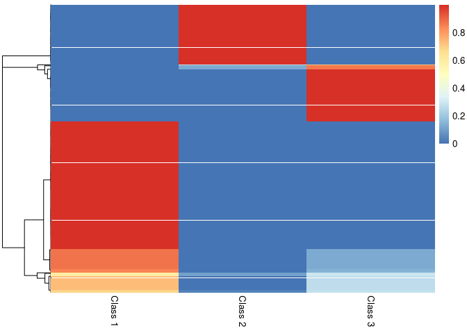
result <- mixdir(mushroom[1:1000, 1:5], n_latent=3)
Analyzing the result
# Latent class of of first 10 mushrooms
head(result$pred_class, n=10)
#>  [1] 3 1 1 3 2 1 1 1 3 1

# Soft Clustering for first 10 mushrooms
head(result$class_prob, n=10)
#>               [,1]         [,2]         [,3]
#>  [1,] 3.103495e-07 1.055098e-05 9.999891e-01
#>  [2,] 9.998594e-01 4.683764e-06 1.359291e-04
#>  [3,] 9.998944e-01 3.111462e-06 1.025194e-04
#>  [4,] 5.778033e-04 7.114603e-08 9.994221e-01
#>  [5,] 3.662625e-07 9.999992e-01 4.183025e-07
#>  [6,] 9.996461e-01 8.764031e-08 3.537838e-04
#>  [7,] 9.998944e-01 3.111462e-06 1.025194e-04
#>  [8,] 9.997331e-01 5.822320e-08 2.668420e-04
#>  [9,] 5.778033e-04 7.114603e-08 9.994221e-01
#> [10,] 9.999999e-01 5.850067e-09 9.845112e-08
pheatmap::pheatmap(result$class_prob, cluster_cols=FALSE,
                  labels_col = paste("Class", 1:3))
# Structure of latent class 1
# (bruises, cap color either yellow or white, edible etc.)
purrr::map(result$category_prob, 1)
#> $bruises
#>      bruises           no
#> 0.9998223256 0.0001776744
#>
#> $`cap-color`
#>        brown         gray          red        white       yellow
#> 0.0001775934 0.0001819672 0.0001776373 0.4079822666 0.5914805356
#>
#> $`cap-shape`
#>      bell    convex      flat    sunken
#> 0.3926736 0.4767291 0.1304197 0.0001776
#>
#> $`cap-surface`
#>   fibrous     scaly    smooth
#> 0.0568571 0.4871396 0.4560033
#>
#> $edible
#>       edible    poisonous
#> 0.9998223174 0.0001776826

# The most predicitive features for each class
find_predictive_features(result, top_n=3)
#>       column    answer class probability
#> 19 cap-color    yellow     1   0.9993990
#> 22 cap-shape      bell     1   0.9990947
#> 1    bruises   bruises     1   0.7089533
#> 48    edible poisonous     3   0.9980468
#> 15 cap-color       red     3   0.8462032
#> 9  cap-color     brown     3   0.6473043
#> 5    bruises        no     2   0.9990364
#> 11 cap-color      gray     2   0.9978218
#> 32 cap-shape    sunken     2   0.9936162
# For example: if all I know about a mushroom is that it has a
# yellow cap, then I am 99% certain that it will be in class 1
predict(result, c(`cap-color`="yellow"))
#>          [,1]         [,2]         [,3]
#> [1,] 0.999399 0.0003004692 0.0003004907

# Note the most predictive features are different from the most typical ones
find_typical_features(result, top_n=3)
#>         column  answer class probability
#> 1      bruises bruises     1   0.9998223
#> 43      edible  edible     1   0.9998223
#> 19   cap-color  yellow     1   0.5914805
#> 3      bruises bruises     3   0.9995546
#> 27   cap-shape  convex     3   0.7460615
#> 9    cap-color   brown     3   0.6746224
#> 44      edible  edible     2   0.9995310
#> 5      bruises      no     2   0.9713177
#> 35 cap-surface fibrous     2   0.7355413
Dimensionality Reduction
# Defining Features
def_feat <- find_defining_features(result, mushroom[1:1000, 1:5], n_features = 3)
print(def_feat)
#> $features
#> [1] "cap-color" "bruises" "edible"
#>
#> $quality
#> [1] 74.35146
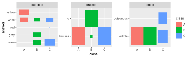
# Plotting the most important features gives an immediate impression
# how the cluster differ
plot_features(def_feat$features, result$category_prob)
#> Loading required namespace: ggplot2
#> Loading required namespace: tidyr
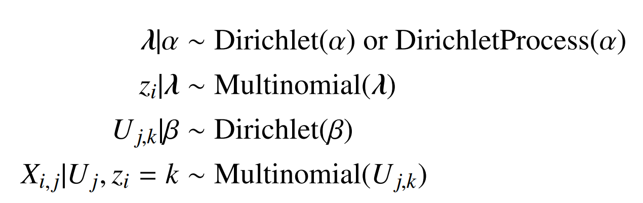
Underlying Model
The package implements a variational inference algorithm to solve a Bayesian latent class model (LCM).