Mongolian 'NSO' 'PXWeb' Data and Boundaries (Tidy Client).

mongolstats

mongolstats is your gateway to the National Statistics Office of Mongolia (NSO). Access official data, analyze economic trends, and map regional statistics—all from within R.

Why mongolstats?

• Instant Access: Query thousands of official datasets directly from R.
• Tidy Data: Analysis-ready tibble format compatible with dplyr and ggplot2.
• Mapping Ready: Built-in administrative boundaries for effortless geospatial analysis.
• Reliable: Smart caching and robust error handling for smooth workflows.

Installation

You can install mongolstats from CRAN with:

install.packages("mongolstats")

Or install the development version from GitHub with:

# install.packages("devtools")
devtools::install_github("temuulene/mongolstats")

Quick Start

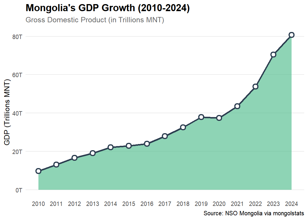
1. The Economic Pulse: GDP Trends

Visualize Mongolia’s economic growth in seconds.

library(mongolstats)
library(dplyr)
library(ggplot2)

# Set language to English
nso_options(mongolstats.lang = "en")

# Fetch GDP data - using labels for clarity
gdp <- nso_data(
  tbl_id = "DT_NSO_0500_001V1",
  selections = list(
    "Indicator" = "GDP, at current prices",
    "Economic activity" = "Total",
    "Year" = c(
      "2010", "2011", "2012", "2013", "2014",
      "2015", "2016", "2017", "2018", "2019",
      "2020", "2021", "2022", "2023", "2024"
    )
  ),
  labels = "en" # Get English labels
)

# Visualize the GDP trend as a static plot
p <- gdp |>
  ggplot(aes(x = as.integer(Year_en), y = value / 1e6, group = 1)) +
  geom_area(fill = "#42b883", alpha = 0.6) +  # shaded area emphasizes cumulative growth
  geom_line(color = "#2c3e50", linewidth = 1.2) +
  geom_point(color = "#2c3e50", size = 3, shape = 21, fill = "white", stroke = 1.5) +
  scale_y_continuous(labels = scales::label_number(suffix = "T")) +  # "T" suffix for trillions
  scale_x_continuous(breaks = function(x) seq(ceiling(min(x)), floor(max(x)), by = 1)) +
  labs(
    title = "Mongolia's GDP Growth (2010-2024)",
    subtitle = "Gross Domestic Product (in Trillions MNT)",
    x = NULL,
    y = "GDP (Trillions MNT)",
    caption = "Source: NSO Mongolia via mongolstats"
  ) +
  theme_minimal(base_size = 12) +
  theme(
    plot.title = element_text(face = "bold", size = 16),
    plot.subtitle = element_text(color = "grey40"),
    panel.grid.minor = element_blank(),
    panel.grid.major.x = element_blank()  # vertical gridlines removed for cleaner look
  )

p  # print static ggplot

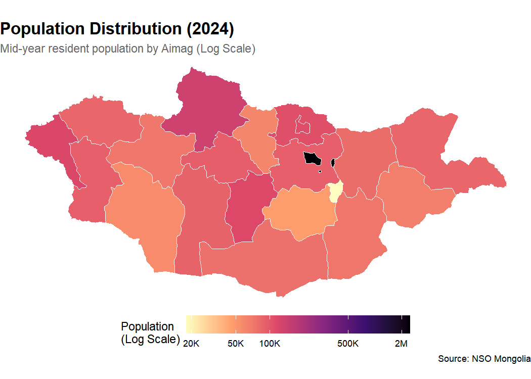
2. Mapping Regional Population

Discover how population is distributed across the country.

library(sf)

# 1. Fetch Population by Aimag
# Get all region codes first
regions <- nso_dim_values("DT_NSO_0300_002V1", "Region")$code

pop <- nso_data(
  tbl_id = "DT_NSO_0300_002V1",
  selections = list(
    "Region" = regions,
    "Year" = "2024" # Use the year label
  ),
  labels = "en" # Get English labels for joining
) |>
  filter(!Region %in% c("0", "1", "2", "3", "4", "511")) |> # Exclude Total, Regions, and duplicate UB
  mutate(
    Region_en = trimws(Region_en),
    Region_en = dplyr::case_match(
      Region_en,
      "Bayan-Ulgii" ~ "Bayan-Ölgii",
      "Uvurkhangai" ~ "Övörkhangai",
      "Khuvsgul" ~ "Hovsgel",
      "Umnugovi" ~ "Ömnögovi",
      "Tuv" ~ "Töv",
      "Sukhbaatar" ~ "Sükhbaatar",
      .default = Region_en
    )
  )

# 2. Get Administrative Boundaries
map <- mn_boundaries(level = "ADM1")

# 3. Join and Map
pop_map <- map |>
  left_join(pop, by = c("shapeName" = "Region_en"))

p <- ggplot(pop_map) +
  geom_sf(aes(fill = value), color = "white", size = 0.2) +
  # Log scale because population spans 3 orders of magnitude (20k to 1.5M)
  scale_fill_viridis_c(
    option = "magma",
    direction = -1,
    trans = "log10",
    breaks = c(20000, 50000, 100000, 500000, 1500000),
    labels = scales::label_number(scale_cut = scales::cut_short_scale()),
    name = "Population\n(Log Scale)"
  ) +
  labs(
    title = "Population Distribution (2024)",
    subtitle = "Mid-year resident population by Aimag (Log Scale)",
    caption = "Source: NSO Mongolia"
  ) +
  theme_void() +
  theme(
    plot.title = element_text(face = "bold", size = 16),
    plot.subtitle = element_text(color = "grey40"),
    legend.position = "bottom",
    legend.key.width = unit(1.5, "cm")
  )

p  # print static ggplot

Documentation

Full documentation is available at temuulene.github.io/mongolstats.

• Getting Started - Your first epidemiological analysis
• Discovery Guide - Find and explore tables
• Mapping Guide - Work with administrative boundaries

Contributing

We welcome contributions! Please see the Contributing Guidelines for details.

License

MIT.