Oblique Random Forests for Right-Censored Time-to-Event Data.
obliqueRSF is deprecated
The aorsf package has superseded obliqueRSF. If you would like to do an analysis with oblique random survival forests, I highly recommend you use aorsf: https://github.com/bcjaeger/aorsf
Overview
Oblique random survival forest (ORSFs) are ensembles for right-censured survival data that use linear combinations of input variables to recursively partition a set of training data. Regularized Cox proportional hazard models identify optimal linear combinations of input variables in each recursive partitioning step while building survival trees.
Installation
You can install obliqueRSF from github with:
# install.packages("devtools")
devtools::install_github("bcjaeger/obliqueRSF")
Usage
The ORSF function is the center piece of the obliqueRSF package
data("pbc",package='survival')

# event is death
# censor study participants at time of last contact or transplant
pbc$status[pbc$status>=1]=pbc$status[pbc$status>=1]-1

# format categorical variables as factors
# if we don't do this, missforest will not impute 0/1 variables
# in the way that we would like it to.
pbc = pbc %>%
  dplyr::select(-id)%>%
  mutate(
    trt=factor(trt),
    ascites=factor(ascites),
    hepato=factor(hepato),
    spiders=factor(spiders),
    edema=factor(edema),
    stage=factor(stage,ordered=TRUE),
    time=time/365.25
  )

orsf <- ORSF(
  data=pbc, # data to fit trees with
  ntree=100, # number of trees to fit
  eval_times=c(1:10), # when will predictions be made?
  # note: eval_times will be used to make figures
  verbose=T,# suppresses console output
  compute_oob_predictions = TRUE # return OOB preds
)
#>
#> performing imputation with missForest:
#>   missForest iteration 1 in progress...done!
#>   missForest iteration 2 in progress...done!
#>   missForest iteration 3 in progress...done!
#>   missForest iteration 4 in progress...done!
#> Fitting tree no. 1
#> Fitting tree no. 2
#> Fitting tree no. 3
#> Fitting tree no. 4
#> Fitting tree no. 5
#> Fitting tree no. 6
#> Fitting tree no. 7
#> Fitting tree no. 8
#> Fitting tree no. 9
#> Fitting tree no. 10
#> Fitting tree no. 11
#> Fitting tree no. 12
#> Fitting tree no. 13
#> Fitting tree no. 14
#> Fitting tree no. 15
#> Fitting tree no. 16
#> Fitting tree no. 17
#> Fitting tree no. 18
#> Fitting tree no. 19
#> Fitting tree no. 20
#> Fitting tree no. 21
#> Fitting tree no. 22
#> Fitting tree no. 23
#> Fitting tree no. 24
#> Fitting tree no. 25
#> Fitting tree no. 26
#> Fitting tree no. 27
#> Fitting tree no. 28
#> Fitting tree no. 29
#> Fitting tree no. 30
#> Fitting tree no. 31
#> Fitting tree no. 32
#> Fitting tree no. 33
#> Fitting tree no. 34
#> Fitting tree no. 35
#> Fitting tree no. 36
#> Fitting tree no. 37
#> Fitting tree no. 38
#> Fitting tree no. 39
#> Fitting tree no. 40
#> Fitting tree no. 41
#> Fitting tree no. 42
#> Fitting tree no. 43
#> Fitting tree no. 44
#> Fitting tree no. 45
#> Fitting tree no. 46
#> Fitting tree no. 47
#> Fitting tree no. 48
#> Fitting tree no. 49
#> Fitting tree no. 50
#> Fitting tree no. 51
#> Fitting tree no. 52
#> Fitting tree no. 53
#> Fitting tree no. 54
#> Fitting tree no. 55
#> Fitting tree no. 56
#> Fitting tree no. 57
#> Fitting tree no. 58
#> Fitting tree no. 59
#> Fitting tree no. 60
#> Fitting tree no. 61
#> Fitting tree no. 62
#> Fitting tree no. 63
#> Fitting tree no. 64
#> Fitting tree no. 65
#> Fitting tree no. 66
#> Fitting tree no. 67
#> Fitting tree no. 68
#> Fitting tree no. 69
#> Fitting tree no. 70
#> Fitting tree no. 71
#> Fitting tree no. 72
#> Fitting tree no. 73
#> Fitting tree no. 74
#> Fitting tree no. 75
#> Fitting tree no. 76
#> Fitting tree no. 77
#> Fitting tree no. 78
#> Fitting tree no. 79
#> Fitting tree no. 80
#> Fitting tree no. 81
#> Fitting tree no. 82
#> Fitting tree no. 83
#> Fitting tree no. 84
#> Fitting tree no. 85
#> Fitting tree no. 86
#> Fitting tree no. 87
#> Fitting tree no. 88
#> Fitting tree no. 89
#> Fitting tree no. 90
#> Fitting tree no. 91
#> Fitting tree no. 92
#> Fitting tree no. 93
#> Fitting tree no. 94
#> Fitting tree no. 95
#> Fitting tree no. 96
#> Fitting tree no. 97
#> Fitting tree no. 98
#> Fitting tree no. 99
#> Fitting tree no. 100
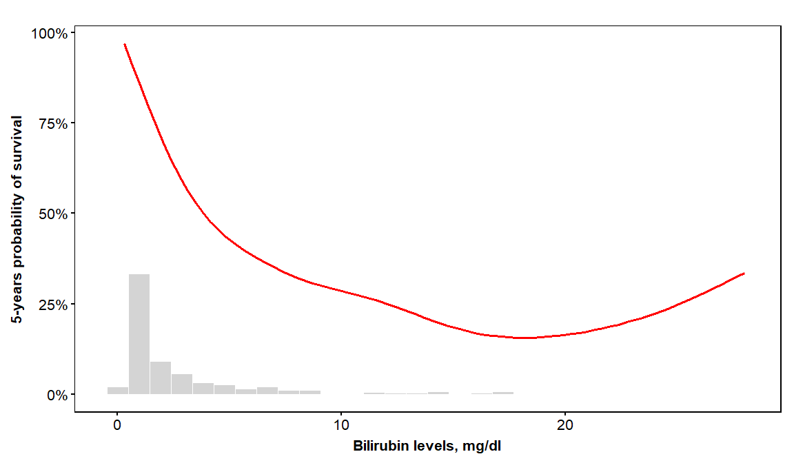
The vdplot function allows you to quickly look at the patterns in the predictions from an ORSF.
# Variable dependence plot (vdplot)

# Survival probabilities for a continuous variable
# note the use of sub_times, which allows you to pick
# one or more times in the evaluation times of an ORSF object

vdplot(object=orsf, xvar='bili', xlab='Bilirubin levels',
       xvar_units = 'mg/dl', sub_times = 5)
#> `stat_bin()` using `bins = 30`. Pick better value with `binwidth`.

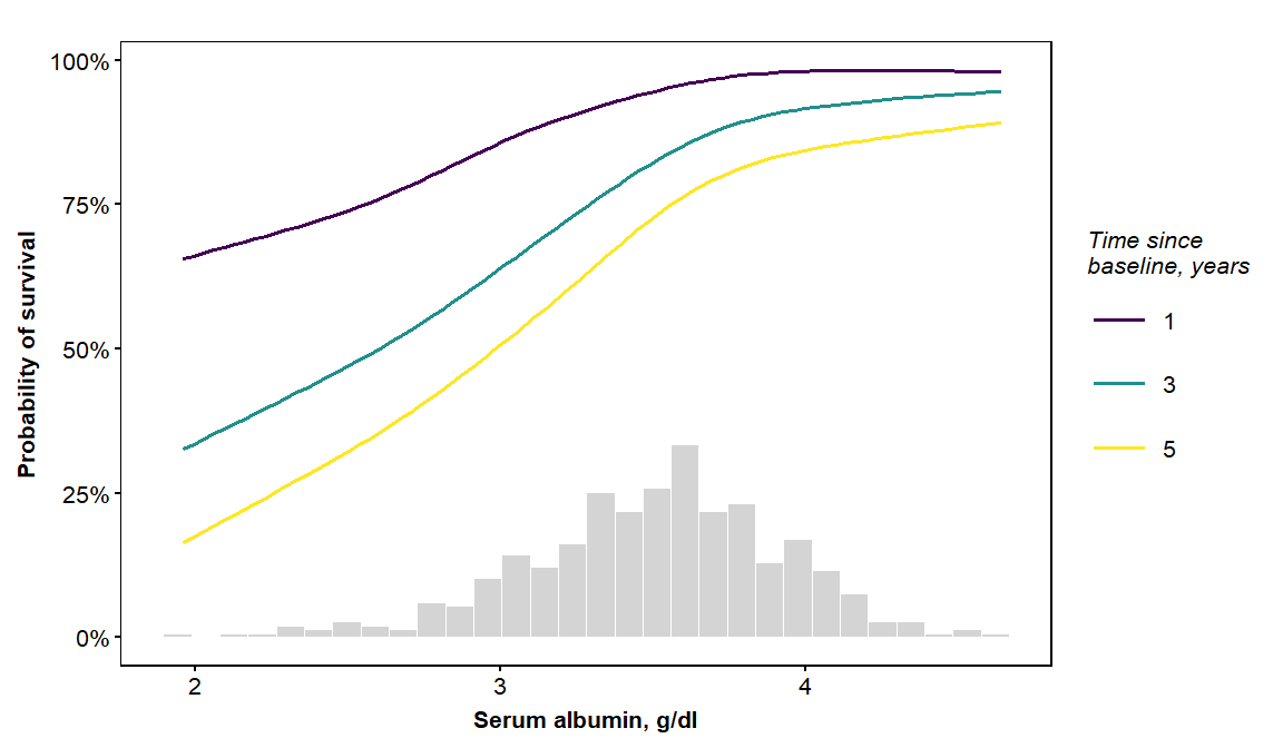
here is another application of vdplot with a continuous x-variable, but this time we will show predictions at three times: 1 year, 3 years, and 5 years since baseline.
vdplot(object=orsf, xvar='albumin', xlab='Serum albumin',
       xvar_units = 'g/dl', sub_times = c(1,3,5))
#> `stat_bin()` using `bins = 30`. Pick better value with `binwidth`.

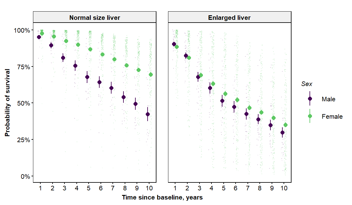
The vdplot function also supports categorical x-variables. Setting the x-variable to sex, and the facet variable to hepato, we find a clear interaction between sex and the presence of an enlarged liver (i.e., hepato=1).
vdplot(object=orsf, xvar='sex', xlab=c("Sex"), xlvls=c("Male","Female"),
       fvar='hepato',flab=c("Normal size liver","Enlarged liver"))
#> Warning: Ignoring unknown parameters: fun.ymin, fun.ymax, fun.y
#> No summary function supplied, defaulting to `mean_se()`
#> No summary function supplied, defaulting to `mean_se()`

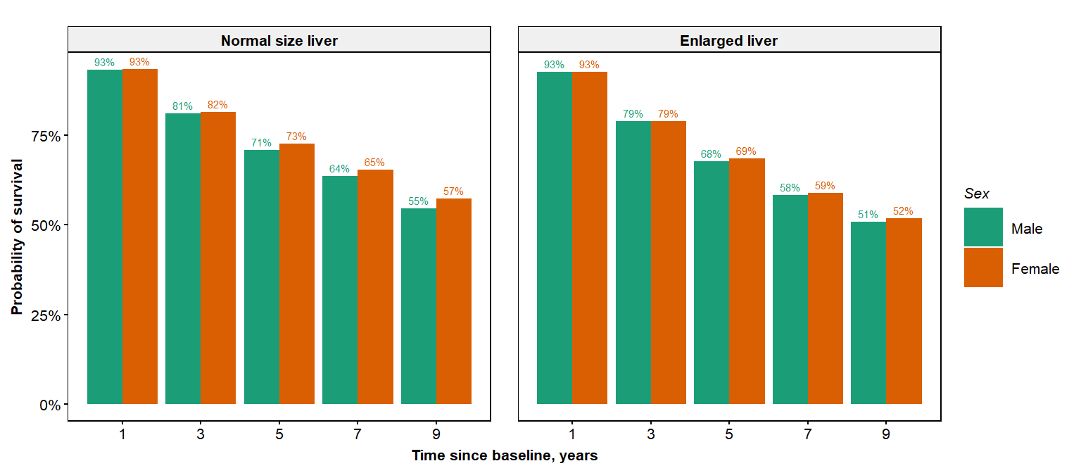
Is this interaction something that is purely explained by sex, or is it a confounding effect from other variables that are not the same between the two sexes? We can address this using the partial dependence plot (pdplot) function:
pdplot(object=orsf, xvar='sex',xlab='Sex', xlvls=c("Male","Female"),
       fvar='hepato',flvls=c("Normal size liver","Enlarged liver"),
       sub_times=c(1,3,5,7,9))
#> Warning: `guides(<scale> = FALSE)` is deprecated. Please use `guides(<scale> =
#> "none")` instead.

Taking into account the effects of other variables in the data, the interaction between sex and hepato is attenuated.