An 'ohsome API' Client.

ohsome: An R package to interact with the ohsome API for OpenStreetMap history data aggregation and extraction

This ohsome R package grants access to the power of the ohsome AP/a from R. ohsome lets you analyze the rich data source of the OpenStreetMap (OSM) history. It aims to leverage the tools of the OpenStreetMap History Database (OSHDB).

With ohsome, you can …

• Get aggregated statistics on the evolution of OpenStreetMap elements and specify your own temporal, spatial and/or thematic filters. The data aggregation endpoint allows you to access functions, e.g., to calculate the area of buildings or the length of streets at any given timestamp.

• Retrieve the geometry of the historical OpenStreetMap data, e.g., to visualize the evolution of certain OpenStreetMap elements over time. You can get the geometries for specific points in time or all changes within a timespan (full-history).

Installation

You can install ohsome from CRAN or from GitHub:

install.packages("ohsome")
remotes::install_github("GIScience/ohsome-r", ref = "main")

Getting started

Upon attaching the ohsome package, a metadata request is sent to the ohsome API. The package message provides some essential metadata information, such as the current temporal extent of the underlying OSHDB:

library(ohsome)
#> Data: © OpenStreetMap contributors https://ohsome.org/copyrights
#> ohsome API version: 1.9.1
#> Temporal extent: 2007-10-08T00:00:00Z to 2023-08-10T20:00Z

The metadata is stored in ohsome_metadata. You can print it to the console to get more details.

You can create any ohsome API query using the generic ohsome_query() function. It takes the endpoint path and any query parameters as inputs. For information on all available endpoints with their parameters, consult the ohsome API documentation or print ohsome_endpoints to the console.

However, this ohsome R package provides specific wrapper functions for queries to all available endpoints.

OSM elements

Aggregating OSM elements

The elements aggregation endpoints of the ohsome API allow querying for the aggregated amount, length, area or perimeter of OpenStreetMap elements with given properties, within given boundaries and at given points in time.

Let us create a query for the total amount of breweries on OSM in the region of Franconia. The first argument to ohsome_elements_count() is the sf object franconia that is included in the mapview package and contains boundary polygons of the 37 districts of the region:

library(mapview)

q <- ohsome_elements_count(franconia, filter = "craft=brewery")

The resulting ohsome_query object can be sent to the ohsome API with ohsome_post(). By default, ohsome_post() returns the parsed API response. In this case, this is a simple data.frame of only one row.

ohsome_post(q, strict = FALSE)
#> Warning: The time parameter is not defined and defaults to the latest available timestamp within the underlying OSHDB.
#> You can use set_time() to set the time parameter.
#>             timestamp value
#> 1 2023-08-10 20:00:00   180

The ohsome_query object was created without an explicit time parameter. When using functions to create element aggregation queries, time defaults to the most recent available timestamp in the underlying OSHDB.[^1]

Defining the time parameter unlocks the full power of ohsome API by giving access to the OSM history. It requires one or more ISO-8601 conform timestring(s). Here is how to create a query for the number of breweries at the first of each month between 2010 and 2020:

ohsome_elements_count(franconia, filter = "craft=brewery", time = "2010/2020/P1M")

Alternatively, we can update the existing ohsome_query object q with the set_time() function, pipe [^2] the modified query directly into ohsome_post() and make a quick visualization with ggplot2:

library(ggplot2)

q |> 
    set_time("2010/2020/P1M") |>
    ohsome_post() |>
    ggplot(aes(x = timestamp, y = value)) +
    geom_line()

This is how to query the total number of breweries in all of Franconia. But what if we want to aggregate the amount per district? The ohsome API provides specific endpoints for different grouped calculations, such as aggregation grouped by bounding geometry.

There are several ways to define a query for an aggregation grouped by boundary:

The set_endpointfunction is used to change or append the endpoint path of an API request. In this case, we could append groupBy/boundary to the existing query to the elements/count endpoint. The endpoint path can either be given as a single string (/groupBy/boundary) or as a character vector: set_endpoint(q, c("groupBy", "boundary"), append = TRUE) [^3].

More comfortable, however, is the use of either the grouping argument with an elements aggregation function (e.g. ohsome_elements_count(grouping = "boundary)) or of the set_grouping() function to modify an existing query object:

library(dplyr)

franconia |> 
    mutate(id = NAME_ASCI) |>
    ohsome_elements_count(filter = "craft=brewery", time = "2021-06-01") |>
    set_grouping("boundary") |>
    ohsome_post()
#> Simple feature collection with 37 features and 3 fields
#> Geometry type: MULTIPOLYGON
#> Dimension:     XY
#> Bounding box:  xmin: 8.975926 ymin: 48.8625 xmax: 12.27535 ymax: 50.56422
#> Geodetic CRS:  WGS 84
#> First 10 features:
#>             groupByBoundaryId value  timestamp                       geometry
#> 1   Bamberg, Kreisfreie Stadt     6 2021-06-01 MULTIPOLYGON (((10.92581 49...
#> 2  Bayreuth, Kreisfreie Stadt     6 2021-06-01 MULTIPOLYGON (((11.58157 49...
#> 3    Coburg, Kreisfreie Stadt     0 2021-06-01 MULTIPOLYGON (((10.95355 50...
#> 4       Hof, Kreisfreie Stadt     1 2021-06-01 MULTIPOLYGON (((11.93067 50...
#> 5          Bamberg, Landkreis    13 2021-06-01 MULTIPOLYGON (((10.87615 50...
#> 6         Bayreuth, Landkreis    13 2021-06-01 MULTIPOLYGON (((11.70656 50...
#> 7           Coburg, Landkreis     6 2021-06-01 MULTIPOLYGON (((10.88654 50...
#> 8                   Forchheim     8 2021-06-01 MULTIPOLYGON (((11.26376 49...
#> 9              Hof, Landkreis     4 2021-06-01 MULTIPOLYGON (((11.91989 50...
#> 10                    Kronach     1 2021-06-01 MULTIPOLYGON (((11.36979 50...

If you want your own identifiers for the geometries returned by ohsome, your input sf object needs a column explicitly named id. You can use mutate() or rename() from the dplyr package to create such a column as in the example below.

By default, ohsome_post() returns an sf object whenever the ohsome API is capable of delivering GeoJSON data. This is the case for elements extraction queries as well as for aggregations grouped by boundaries.

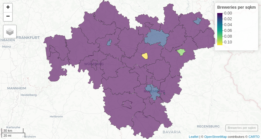
Thus, you can easily create a choropleth map from the query results. In addition, you can set the argument return_value to density. This will modify the endpoint path of the query so that ohsome returns the number of breweries per area instead of the absolute value:

franconia |> 
    mutate(id = NAME_ASCI) |>
    ohsome_elements_count(filter = "craft=brewery", return_value = "density") |>
    set_time("2021-06-01") |>
    set_grouping("boundary") |>
    ohsome_post() |>
    mapview(zcol = "value", layer.name = "Breweries per sqkm")

Extracting OSM elements

The elements extraction endpoints of the ohsome API allow obtaining geometries, bounding boxes or centroids of OSM elements with given properties, within given boundaries and at given points in time. Together with the elements, you can choose to query for their tags and/or their metadata such as the changeset ID, the time of the last edit or the version number.

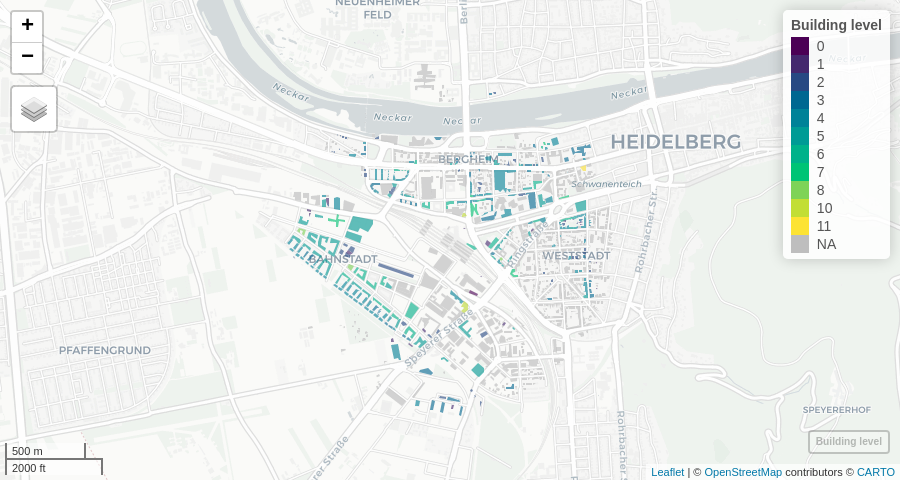
The following query extracts the geometries of buildings within 1000 m of Heidelberg main station with their tags. The response is used to visualize the buildings and the values of their building:levels tag (if available):

hd_station_1km <- ohsome_boundary("8.67542,49.40347,1000")

ohsome_elements_geometry(
    boundary = hd_station_1km, 
    filter = "building=* and type:way", 
    time = "2021-12-01",
    properties = "tags", 
    clipGeometry = FALSE
) |>
    ohsome_post() |>
    transmute(level = factor(`building:levels`)) |>
    mapview(zcol = "level", lwd = 0, layer.name = "Building level")

Similarly, you can use ohsome_elements_centroid() to extract centroids of OSM elements and ohsome_elements_bbox() for their bounding boxes. Note that OSM node elements (with point geometries) are omitted from the results if querying for bounding boxes.

Extracting the full history of OSM elements

While the elements extraction endpoints provide geometries and properties of OSM elements at specific timestamps, results of queries to the full history endpoints will include all changes to matching OSM features with corresponding validFrom and validTo timestamps.

Here, we request the full history of OSM buildings within 1000 m of Heidelberg main station, filter for features that still exist and visualize all building features with their year of creation:

meta <- ohsome_get_metadata()
start <- meta$extractRegion$temporalExtent[1]
end <- "2023-01-01"

ohsome_elementsFullHistory_geometry(
    boundary = hd_station_1km,
    time = c(start, end),
    filter = "building=* and geometry:polygon", 
    clipGeometry = FALSE,
    properties = "metadata"
) |> 
    ohsome_post() |>
    janitor::clean_names() |>
    group_by(osm_id) |>
    mutate(year = min(format(valid_from, "%Y"))) |>
    filter(valid_to == lubridate::ymd(end)) |>
    mapview(zcol = "year", lwd = 0, layer.name = "Year of Feature Creation")

You may find using clean_names() from the janitor package helpful in order to remove special characters from column names in the parsed ohsome API response – just as in the example above.

OSM contributions

Aggregating OSM contributions

With queries to the ohsome API’s contributions aggregation endpoints, you can get counts of the contributions provided by users to OSM. The following code requests the number of deletions of man-made objects at the location of the hypothetical Null Island per year between 2010 and 2020:

ohsome_contributions_count(
    boundary = "0,0,10", 
    filter = "man_made=*", 
    time = "2010/2020/P1Y",
    contributionType = "deletion"
) |>
    ohsome_post()
#>    fromTimestamp toTimestamp value
#> 1     2010-01-01  2011-01-01     0
#> 2     2011-01-01  2012-01-01     1
#> 3     2012-01-01  2013-01-01     0
#> 4     2013-01-01  2014-01-01     0
#> 5     2014-01-01  2015-01-01     0
#> 6     2015-01-01  2016-01-01     3
#> 7     2016-01-01  2017-01-01     1
#> 8     2017-01-01  2018-01-01     8
#> 9     2018-01-01  2019-01-01     4
#> 10    2019-01-01  2020-01-01     4

The contributionType parameter is used to filter for specific types of contributions (in this case: deletions). If it is not set, any contribution is counted. Note that the resulting values apply to time intervals defined by a fromTimestamp and a toTimestamp.

Extracting OSM contributions

The contributions extraction endpoints of the ohsome API can be used to extract feature geometries of contributions.

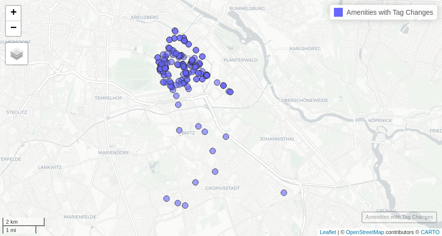
In the following example, we extract the centroids of all amenities in the Berlin city district of Neukölln that have had contributions in March 2020. Consequently, we filter for features that have had tags changed and visualize their locations:

nominatimlite::geo_lite_sf("Berlin Neukoelln", points_only = FALSE) |>
    ohsome_contributions_centroid() |>
    set_filter("amenity=*") |>
    set_time("2020-03,2020-04") |>
    set_properties("contributionTypes") |> 
    ohsome_post() |>
    filter(`@tagChange`) |>
    mapview(layer.name = "Amenities with Tag Changes")
#> Warning: 60 element(s) with empty geometries omitted.

OSM users

You can get statistics on the number of users editing specific features through the users aggregation endpoints of the ohsome API.

Here, we show the number of users editing buildings before, during and after the Nepal earthquake 2015:

ohsome_users_count(
    boundary = "82.3055,6.7576,87.4663,28.7025",
    filter = "building=* and geometry:polygon",
    time = "2015-03-01/2015-08-01/P1M"
) |>
    ohsome_post()
#>   fromTimestamp toTimestamp value
#> 1    2015-03-01  2015-04-01    97
#> 2    2015-04-01  2015-05-01  3489
#> 3    2015-05-01  2015-06-01  3103
#> 4    2015-06-01  2015-07-01   478
#> 5    2015-07-01  2015-08-01   185

Bounding geometries

The ohsome API requires bounding geometries either as bounding polygons (bpolys), bounding boxes (bboxes) or bounding circles (bcircles) parameters to the query in a textual form (see ohsome API documentation). The ohsome R package uses the generic function ohsome_boundary() under the hood to make your life easier. It accepts a wider range of input geometry formats, while guessing the right type of bounding geometry.

As seen above, sf objects can be passed into the boundary argument of ohsome_query() and any of its wrapper functions. You can also update queries with set_boundary(). The sf object will be converted into GeoJSON and passed into the bpolys parameter of the query.

If you wish to aggregate or extract OSM elements on administrative boundaries in the sf format, you might want to check out packages such as rnaturalearth, geodata, raster (in particular its getData() function), rgeoboundaries or nominatimlite for the acquisition of boundary data that can be used with ohsome_boundary().

There are also the following methods of ohsome_boundary() for other classes of input geometry objects:

1. bbox objects created with st_bbox are converted into a textual bboxes parameter to the query:

q <- ohsome_query("users/count") |>
    set_boundary(sf::st_bbox(franconia))

q$body$bboxes
#> [1] "8.97592600000002,48.862505,12.2753535,50.5642245"

2. matrix objects created with sp::bbox(), raster::bbox() or terra::bbox() are also converted into a textual bboxes parameter. This even applies for matrices created with osmdata::getbb() and tmaptools::bb(), so that you can comfortably acquire bounding boxes from the Nominatim API:

osmdata::getbb("Kigali") |> 
    ohsome_elements_length(time = "2018/2018-12/P1M", filter = "route=bus") |>
    ohsome_post()
#>     timestamp     value
#> 1  2018-01-01  28251.24
#> 2  2018-02-01  28251.24
#> 3  2018-03-01  29103.11
#> 4  2018-04-01 186645.71
#> 5  2018-05-01 378185.54
#> 6  2018-06-01 473065.23
#> 7  2018-07-01 615801.98
#> 8  2018-08-01 648385.19
#> 9  2018-09-01 753618.88
#> 10 2018-10-01 771239.17
#> 11 2018-11-01 847337.73
#> 12 2018-12-01 858886.63

3. You can pass any character object with text in the format allowed by the ohsome AP/a to ohsome_boundary() – even GeoJSON FeatureCollections. It will automatically detect whether you have passed the definition of bpolys, bboxes or bcircles. It is possible to use character vectors where each element represents one geometry:

c("Circle 1:8.6528,49.3683,1000", "Circle 2:8.7294,49.4376,1000") |>
    ohsome_elements_count(filter = "amenity=*", grouping = "boundary", time = 2021) |>
    ohsome_post()
#> Simple feature collection with 2 features and 3 fields
#> Geometry type: POLYGON
#> Dimension:     XY
#> Bounding box:  xmin: 8.639026 ymin: 49.35931 xmax: 8.743193 ymax: 49.44659
#> Geodetic CRS:  WGS 84
#>   groupByBoundaryId value  timestamp                       geometry
#> 1          Circle 1    16 2021-01-01 POLYGON ((8.666574 49.36834...
#> 2          Circle 2    20 2021-01-01 POLYGON ((8.743193 49.43763...

⚠️ While sf and bbox objects will be automatically transformed to WGS 84 if in a different coordinate reference system, coordinates in character and matrix objects always need to be provided as WGS 84.

Modifying queries

As seen above, existing ohsome_query objects can be modified by set_endpoint(), set_grouping(), set_boundary() or set_time(). The latter and other functions such as set_filter() are just wrappers around the more generic set_parameters(). This can be used to modify the parameters of a query in any possible way:

q <- ohsome_elements_count("8.5992,49.3567,8.7499,49.4371")

q |>
    set_endpoint("ratio", append = TRUE) |>
    set_parameters(
        filter = "building=*", 
        filter2 = "building=* and building:levels=*",
        time = "2010/2020/P2Y"
    ) |>
    ohsome_post()
#>    timestamp value value2    ratio
#> 1 2010-01-01   554      3 0.005415
#> 2 2012-01-01 10600      7 0.000660
#> 3 2014-01-01 21005     77 0.003666
#> 4 2016-01-01 25849    798 0.030872
#> 5 2018-01-01 29397   1223 0.041603
#> 6 2020-01-01 31495   1456 0.046230

Grouping

Grouping endpoints are available for aggregation resources and can be used to compute the aggregated results grouped by:

• boundary,
• key,
• tag, and
• type.

In many cases, a grouping by boundary can be combined with a grouping by tag. Some of the grouping endpoints require additional query parameters, e.g. tag groupings require a groupByKey parameter. Not all grouping endpoints are available for all aggregation resources – please consult the ohsome API documentation for details.

You can set the grouping argument to any aggregation endpoint wrapper function (e.g. ohsome_elements_count(grouping = c("boundary", "tag"))) or use set_grouping() to modify existing query objects.

Density and ratio requests

Many aggregation resources have endpoints for requesting density (i.e. count, length, perimeter or area of features per area) or ratios (of OSM elements satisfying a filter2 to elements satisfying a filter) instead of or in addition to absolute values.

You can request density or ratio values by setting the return_value argument to aggregation endpoint wrapper functions (e.g. ohsome_elements_count(return_value = "density")). Mind that ratio endpoints require an additional filter2 query parameter. Please consult the ohsome API documentation or print names(ohsome_endpoints) to the console in order to check for the availability of specific density and ratio endpoints.

Dealing with complex API responses

The ohsome API allows grouping aggregate values for various timestamps by boundary and tag at the same time. The parsed content of the response can be rather complex. In the following case, building feature counts for the districts of Franconia at two different timestamps are requested – additionally grouped by the building:levels tag. To avoid lots of redundant geometries, comma-separated values (instead of GeoJSON) are explicitly requested as the response format:

building_levels <- franconia |>
    mutate(id  = NUTS_ID) |>
    ohsome_elements_count(grouping = c("boundary", "tag"), format = "csv") |>
    set_filter("building=* and geometry:polygon") |>
    set_time("2015/2020") |>
    set_groupByKey("building:levels") |>
    ohsome_post()

dim(building_levels)
#> [1]    2 1999

The query results in a confusing data.frame with 1999 columns and 2 rows. This happens because there is a building count column for each combination of boundary polygon and number of levels, while the two requested timestamps are in the rows. Fortunately, there is the tidyr package to do its magic and pivot this table into a long format with one value per row:

library(tidyr)

building_levels |>
    pivot_longer(-timestamp, names_to = c("id", "levels"), names_sep = "_")
#> # A tibble: 3,996 × 4
#>    timestamp           id    levels            value
#>    <dttm>              <chr> <chr>             <dbl>
#>  1 2015-01-01 00:00:00 DE241 remainder          4307
#>  2 2015-01-01 00:00:00 DE241 building.levels.1  6347
#>  3 2015-01-01 00:00:00 DE241 building.levels.2  6727
#>  4 2015-01-01 00:00:00 DE241 building.levels.3  2787
#>  5 2015-01-01 00:00:00 DE241 building.levels.4   745
#>  6 2015-01-01 00:00:00 DE241 building.levels.5    96
#>  7 2015-01-01 00:00:00 DE241 building.levels.6    38
#>  8 2015-01-01 00:00:00 DE241 building.levels.9     7
#>  9 2015-01-01 00:00:00 DE241 building.levels.0     0
#> 10 2015-01-01 00:00:00 DE241 building.levels.7    32
#> # ℹ 3,986 more rows

How to cite this package

In order to cite this package in publications, please use the citation information provided through citation("ohsome").

[^1]: ohsome_post fails on queries created with an undefined time parameter unless strict query validation is disabled with strict = FALSE.

[^2]: Instead of the new R native pipe |> you may choose to use magrittr’s %>%.

[^3]: The order of the elements in the character vector is critical!