Agglomerative Partitioning Framework for Dimension Reduction.

partition

partition is a fast and flexible framework for agglomerative partitioning. partition uses an approach called Direct-Measure-Reduce to create new variables that maintain the user-specified minimum level of information. Each reduced variable is also interpretable: the original variables map to one and only one variable in the reduced data set. partition is flexible, as well: how variables are selected to reduce, how information loss is measured, and the way data is reduced can all be customized.

Installation

You can install the partition from CRAN with:

install.packages("partition")

Or you can install the development version of partition GitHub with:

# install.packages("remotes")
remotes::install_github("USCbiostats/partition")

Example

library(partition)
set.seed(1234)
df <- simulate_block_data(c(3, 4, 5), lower_corr = .4, upper_corr = .6, n = 100)

#  don't accept reductions where information < .6
prt <- partition(df, threshold = .6)
prt
#> Partitioner:
#>    Director: Minimum Distance (Pearson) 
#>    Metric: Intraclass Correlation 
#>    Reducer: Scaled Mean
#> 
#> Reduced Variables:
#> 1 reduced variables created from 2 observed variables
#> 
#> Mappings:
#> reduced_var_1 = {block2_x3, block2_x4}
#> 
#> Minimum information:
#> 0.602

# return reduced data
partition_scores(prt)
#> # A tibble: 100 × 11
#>    block1_x1 block1_x2 block1_x3 block2_x1 block2_x2 block3_x1 block3_x2
#>        <dbl>     <dbl>     <dbl>     <dbl>     <dbl>     <dbl>     <dbl>
#>  1   -1.00     -0.344      1.35     -0.526    -1.25      1.13     0.357 
#>  2    0.518    -0.434     -0.361    -1.48     -1.53     -0.317    0.290 
#>  3   -1.77     -0.913     -0.722     0.122     0.224    -0.529    0.114 
#>  4   -1.49     -0.998      0.189     0.149    -0.994    -0.433    0.0120
#>  5    0.616     0.0211     0.895     1.09     -1.25      0.440   -0.550 
#>  6    0.0765    0.522      1.20     -0.152    -0.419    -0.912   -0.362 
#>  7    1.74      0.0993    -0.654    -1.26     -0.502    -0.792   -1.03  
#>  8    1.05      2.19       0.913     0.254     0.328    -1.07    -0.976 
#>  9   -1.07     -0.292     -0.763     0.437     0.739     0.899   -0.342 
#> 10   -1.02     -0.959     -1.33     -1.57     -1.11      0.618    0.153 
#> # ℹ 90 more rows
#> # ℹ 4 more variables: block3_x3 <dbl>, block3_x4 <dbl>, block3_x5 <dbl>,
#> #   reduced_var_1 <dbl>

# access mapping keys
mapping_key(prt)
#> # A tibble: 11 × 4
#>    variable      mapping   information indices  
#>    <chr>         <list>          <dbl> <list>   
#>  1 block1_x1     <chr [1]>       1     <int [1]>
#>  2 block1_x2     <chr [1]>       1     <int [1]>
#>  3 block1_x3     <chr [1]>       1     <int [1]>
#>  4 block2_x1     <chr [1]>       1     <int [1]>
#>  5 block2_x2     <chr [1]>       1     <int [1]>
#>  6 block3_x1     <chr [1]>       1     <int [1]>
#>  7 block3_x2     <chr [1]>       1     <int [1]>
#>  8 block3_x3     <chr [1]>       1     <int [1]>
#>  9 block3_x4     <chr [1]>       1     <int [1]>
#> 10 block3_x5     <chr [1]>       1     <int [1]>
#> 11 reduced_var_1 <chr [2]>       0.602 <int [2]>

unnest_mappings(prt)
#> # A tibble: 12 × 4
#>    variable      mapping   information indices
#>    <chr>         <chr>           <dbl>   <int>
#>  1 block1_x1     block1_x1       1           1
#>  2 block1_x2     block1_x2       1           2
#>  3 block1_x3     block1_x3       1           3
#>  4 block2_x1     block2_x1       1           4
#>  5 block2_x2     block2_x2       1           5
#>  6 block3_x1     block3_x1       1           8
#>  7 block3_x2     block3_x2       1           9
#>  8 block3_x3     block3_x3       1          10
#>  9 block3_x4     block3_x4       1          11
#> 10 block3_x5     block3_x5       1          12
#> 11 reduced_var_1 block2_x3       0.602       6
#> 12 reduced_var_1 block2_x4       0.602       7

# use a lower threshold of information loss
partition(df, threshold = .5, partitioner = part_kmeans())
#> Partitioner:
#>    Director: <custom director> 
#>    Metric: <custom metric> 
#>    Reducer: <custom reducer>
#> 
#> Reduced Variables:
#> 2 reduced variables created from 7 observed variables
#> 
#> Mappings:
#> reduced_var_1 = {block3_x1, block3_x2, block3_x5}
#> reduced_var_2 = {block2_x1, block2_x2, block2_x3, block2_x4}
#> 
#> Minimum information:
#> 0.508

# use a custom partitioner
part_icc_rowmeans <- replace_partitioner(
  part_icc, 
  reduce = as_reducer(rowMeans)
)
partition(df, threshold = .6, partitioner = part_icc_rowmeans) 
#> Partitioner:
#>    Director: Minimum Distance (Pearson) 
#>    Metric: Intraclass Correlation 
#>    Reducer: <custom reducer>
#> 
#> Reduced Variables:
#> 1 reduced variables created from 2 observed variables
#> 
#> Mappings:
#> reduced_var_1 = {block2_x3, block2_x4}
#> 
#> Minimum information:
#> 0.602

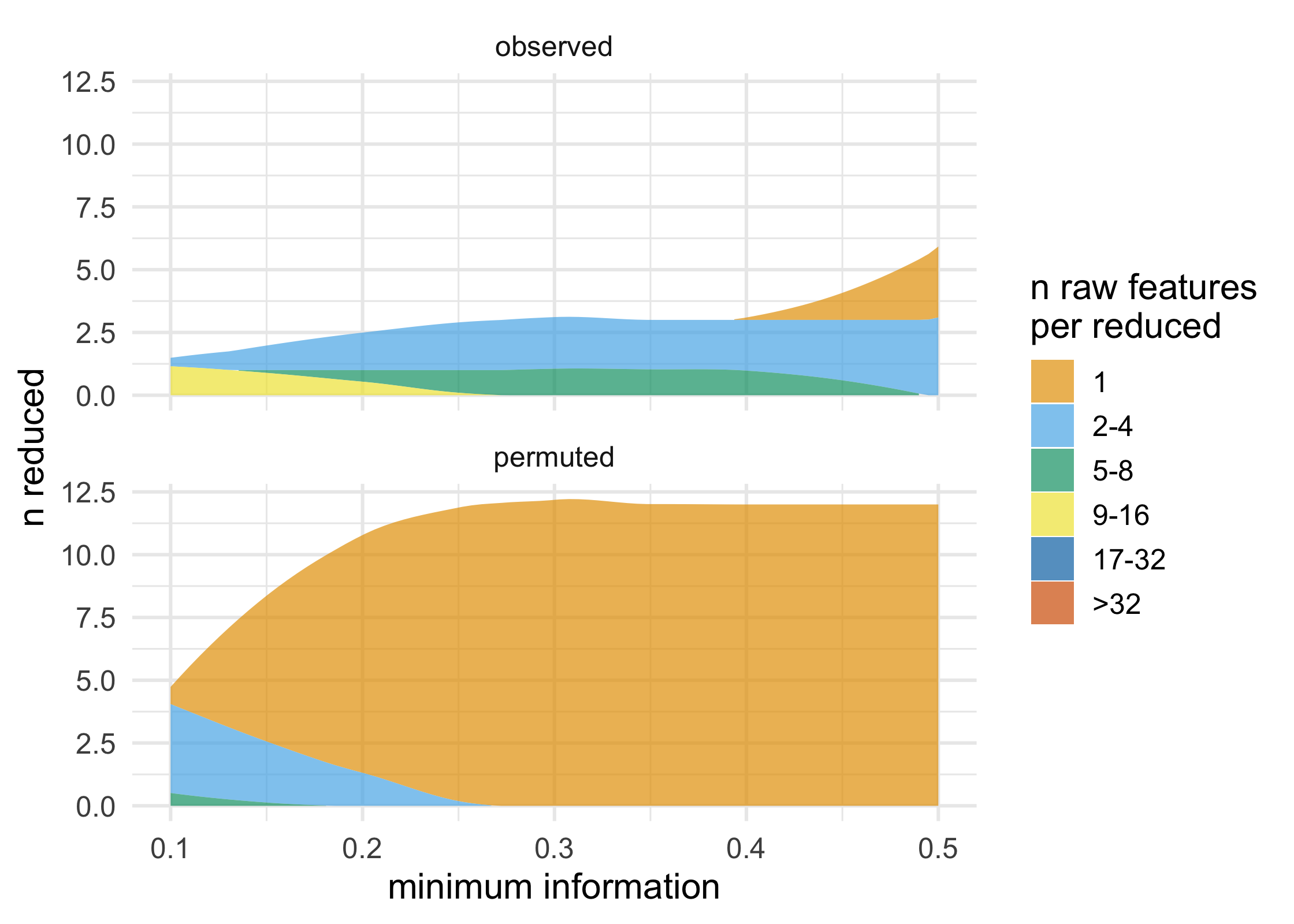
partition also supports a number of ways to visualize partitions and permutation tests; these functions all start with plot_*(). These functions all return ggplots and can thus be extended using ggplot2.

plot_stacked_area_clusters(df) +
  ggplot2::theme_minimal(14)

Performance

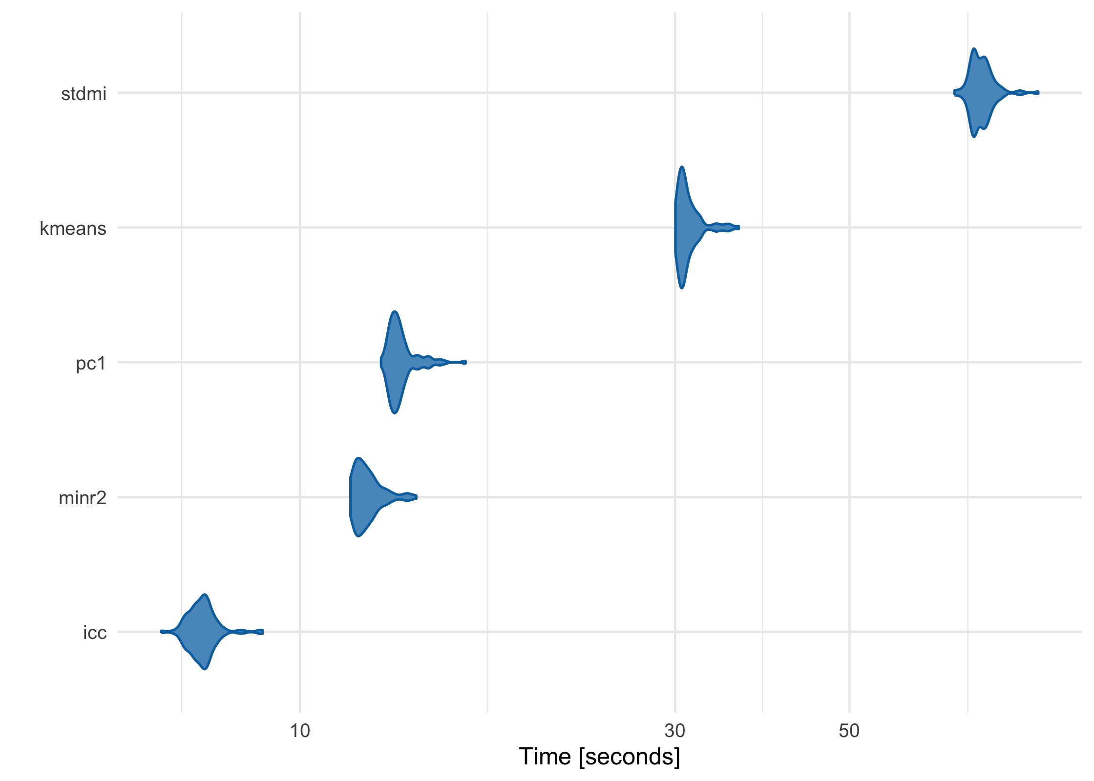
partition has been meticulously benchmarked and profiled to improve performance, and key sections are written in C++ or use C++-based packages. Using a data frame with 1 million rows on a 2017 MacBook Pro with 16 GB RAM, here’s how each of the built-in partitioners perform:

large_df <- simulate_block_data(c(3, 4, 5), lower_corr = .4, upper_corr = .6, n = 1e6)

basic_benchmarks <- microbenchmark::microbenchmark(
  icc = partition(large_df, .3),
  kmeans = partition(large_df, .3, partitioner = part_kmeans()),
  minr2 = partition(large_df, .3, partitioner = part_minr2()),
  pc1 = partition(large_df, .3, partitioner = part_pc1()),
  stdmi = partition(large_df, .3, partitioner = part_stdmi())
)

ICC vs K-Means

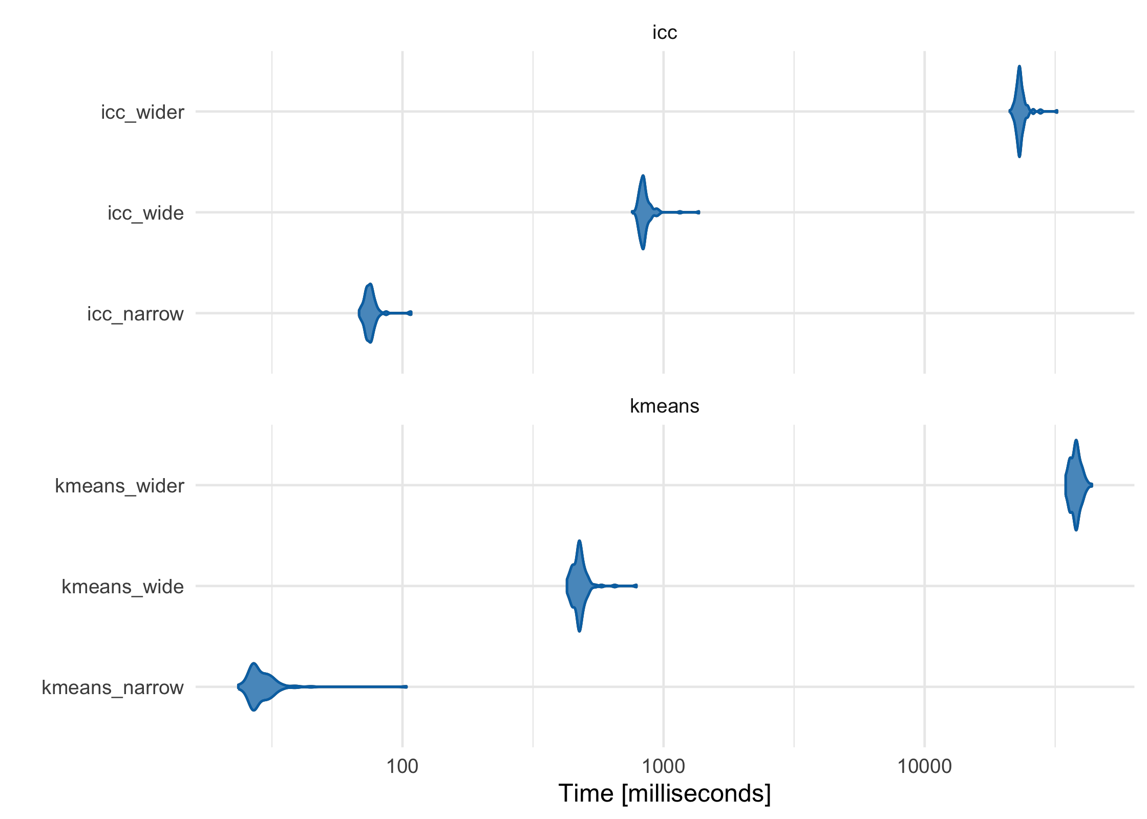
As the features (columns) in the data set become greater than the number of observations (rows), the default ICC method scales more linearly than K-Means-based methods. While K-Means is often faster at lower dimensions, it becomes slower as the features outnumber the observations. For example, using three data sets with increasing numbers of columns, K-Means starts as the fastest and gets increasingly slower, although in this case it is still comparable to ICC:

narrow_df <- simulate_block_data(3:5, lower_corr = .4, upper_corr = .6, n = 100)
wide_df <- simulate_block_data(rep(3:10, 2), lower_corr = .4, upper_corr = .6, n = 100)
wider_df <- simulate_block_data(rep(3:20, 4), lower_corr = .4, upper_corr = .6, n = 100)

icc_kmeans_benchmarks <- microbenchmark::microbenchmark(
  icc_narrow = partition(narrow_df, .3),
  icc_wide = partition(wide_df, .3),
  icc_wider = partition(wider_df, .3),
  kmeans_narrow = partition(narrow_df, .3, partitioner = part_kmeans()),
  kmeans_wide = partition(wide_df, .3, partitioner = part_kmeans()),
  kmeans_wider  = partition(wider_df, .3, partitioner = part_kmeans())
)

For more information, see our paper in Bioinformatics, which discusses these issues in more depth (Millstein et al. 2020).

Contributing

Please read the Contributor Guidelines prior to submitting a pull request to partition. Also note that this project is released with a Contributor Code of Conduct. By participating in this project you agree to abide by its terms.

References

Millstein, Joshua, Francesca Battaglin, Malcolm Barrett, Shu Cao, Wu Zhang, Sebastian Stintzing, Volker Heinemann, and Heinz-Josef Lenz. 2020. “Partition: A Surjective Mapping Approach for Dimensionality Reduction.” Bioinformatics 36 (3): 676–81. https://doi.org/10.1093/bioinformatics/btz661.