Calculate a Piecewise Normalised Score Using Class Intervals.

piecenorm

The goal of piecenorms is to provide implementation of piecewise normalisation techniques useful when dealing with the communication of skewed and highly skewed data.

Installation

You can install the development version of piecenorm from GitHub with:

install.packages('piecenorms')
# install.packages("devtools")
devtools::install_github("david-hammond/piecenorm")

Example

This is a basic example which shows you how to solve a common normalisation problem. There are many mathematical transformations that can be made on skewed data. However, these can be a barrier when communicating to a non-technical audience. piecenorms allows the use to:

1. Provide a set of observations obs

2. Select a set of class breaks, either through using the classInt (or other similar) packages, or by selecting the manually based on expert judgement and ease of communication purposes.

3. Calculate a normalisation of between 0 and 1 for the values within the observations based on the class intervals.

Example R Code can be found below.

set.seed(12345)
library(piecenorms)
x <- round(exp(1:10),2)
brks <- c(min(x), 8, 20, 100, 1000, 25000)
y <- piecenorm(x, brks)
#> Note: Maximum of the breaks is greater than
#>             the maximum of the observations.
#> Proceeding with calculation, normalised values
#>             will have a maximum < 1
plot(x, y, type = 'l',
     xlab = "Original Values",
     ylab = "Normalised Values")

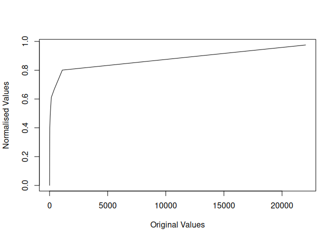
For any call to piecenorm, the user provides a vector of observations, a vector of breaks and a direction for the normalisation. The data is then cut into classes and normalised within its class.

Number of Bins:

$$\begin{equation}{ n = \text{length}(\text{brks}) - 1}\end{equation}$$

Normalisation Class Intervals:

$$\begin{equation}{\left(\frac{i-1}{n}, \frac{i}{n}\right] \forall i \in {1:n}}\end{equation}$$

In cases where there is only one bin defined as c(min(obs), max(obs)), the function piecenorm resolves to standard minmax normalisation.

Notes

As with any non-linear transformation, piecewise normalization preserves ordinal invariance within each class but does not preserve global relative magnitudes. However, it does maintain relative magnitudes within each class. On the other hand, more standard techniques like min-max normalization preserves both ordinal invariance and global relative magnitudes.

Definitions of each are as follows:

• Ordinal Invariance: The property that the order of the data points is preserved. If one normalized value is larger than another, it reflects the same order as in the original data.

• Non-Preservation of Relative Magnitudes (Global): This refers to the loss of the proportionality of the original data values when normalized. If one value is twice as large as another in the original data, this relationship might not be preserved in the normalized data.

• Within-Class Relative Magnitude Preservation: This indicates that within each class or subset of data, the relative magnitudes of the data points are maintained. If data points are normalized within classes, their relative sizes in relation to each other remain the same as in the original data.

normalisr R6 class

piecenorms also provides a normalisr R6 class that

• Classifies the distribution of user data
• Recommends a piecewise normalisation technique
• Calculates normalised data and the percentiles
• Provides plot(), print(), hist() and as.data.frame() methods to allow comparison of original and normalised data.
• Provides the user the ability to set Manual normalisation breaks via SetManualBreaks(). This is useful when manual breaks are easier to communicate to a non-technical audience.
• Provides an applyto() method that allows the normalisr breask to be applied to different data. Useful when user wished to analyse howe normalised values have changed over time.

An example is provided below:

# Lognormal distribution test
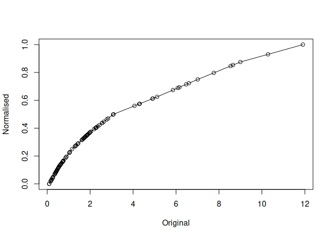
x <- rlnorm(100)
y <- rlnorm(100)
mdl <- normalisr$new(x)
print(mdl)
#> Likely Distribution: 
#> [1] "Lognormal"
#> Suggested Normalisation: 
#> [1] "jenks"
#> Suggested Breaks: 
#> [1]  0.09251744  0.55605971  1.16136029  2.03290543  3.09104998  5.11637223
#> [7]  7.01248874  8.99648141 11.90681490
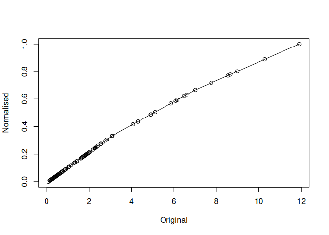
mdl$plot()

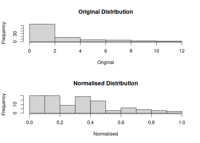
mdl$hist()

head(mdl$as.data.frame())
#>       value percentile bins            int normalised
#> 1 1.7959405 0.57575758    4    (1.16,2.03] 0.34101367
#> 2 2.0329054 0.66666667    4    (1.16,2.03] 0.37500000
#> 3 0.8964585 0.39393939    3   (0.556,1.16] 0.19529540
#> 4 0.6354021 0.29292929    3   (0.556,1.16] 0.14138493
#> 5 1.8328781 0.58585859    4    (1.16,2.03] 0.34631139
#> 6 0.1623573 0.03030303    2 (0.0925,0.556] 0.01883319
mdl$applyto(y)
#> Note: Minimum of the breaks is lower than the
#>             minimum of the observations.
#> Proceeding with calculation, normalised
#>             values will have a minimum > 0
#> Note: Truncating observations outside of the breaks.
#> Likely Distribution: 
#> [1] "Lognormal"
#> Suggested Normalisation: 
#> [1] "jenks"
#> Suggested Breaks: 
#> [1]  0.09251744  0.55605971  1.16136029  2.03290543  3.09104998  5.11637223
#> [7]  7.01248874  8.99648141 11.90681490

# Lognormal distribution test with 3 classes
mdl <- normalisr$new(x, num_classes = 3)
print(mdl)
#> Likely Distribution: 
#> [1] "Lognormal"
#> Suggested Normalisation: 
#> [1] "jenks"
#> Suggested Breaks: 
#> [1]  0.09251744  3.09104998  7.01248874 11.90681490
mdl$plot()

mdl$hist()