Calculate Crosstab and Topline Tables of Weighted Survey Data.
Weighted data survey tables in R
John Johnson 3/9/2020
pollster is an R package for making topline and crosstab tables of simple weighted survey data. The package is designed for use with labelled data, like what you might use the haven package to import from Stata or SPSS. It follows tidyverse programming conventions, and output tables are also in the form of a tidy data frame, or tibble.
Only simple weights are currently supported. For complex survey designs, we recommend the excellent survey package.
The core functions are:
topline()crosstab()crosstab_3way()
Each of these functions also has a twin version which includes a column for the margin of error calculated to include the design effect of the weights.
moe_topline()moe_crosstab()moe_crosstab_3way()
There are also two special functions which calculate the design effect component of the margin of error for each survey wave independently.
moe_wave_crosstab()moe_wave_crosstab_3way()
Other functions are included to calculate simple weighted summary statistics.
wtd_mean()is a tidy-compliant wrapper aroundstats::weighted.mean()summary_table()returns a tible with summary statistics similar to the Stata commandsum
Installation
Install it this way.
install.packages("pollster")
Or get the development version.
remotes::install_github("jdjohn215/pollster")
Basic usage
pollster includes a dataset of Illinois responses to the Current Population Survey’s voter registration supplement.
library(pollster)
head(illinois)
#> # A tibble: 6 x 10
#>    year    fips     sex   educ6 raceethnic maritalstatus      rv   voter   age
#>   <dbl> <dbl+l> <dbl+l> <dbl+l>  <dbl+lbl>     <dbl+lbl> <dbl+l> <dbl+l> <dbl>
#> 1  1996 17 [IL] 1 [Mal… 2 [HS]   1 [White] 1 [Married]   2 [Not… 2 [Not…    29
#> 2  1996 17 [IL] 2 [Fem… 3 [Som…  1 [White] 1 [Married]   1 [Reg… 1 [Vot…    28
#> 3  1996 17 [IL] 2 [Fem… 2 [HS]   1 [White] 3 [Never Mar… 1 [Reg… 1 [Vot…    82
#> 4  1996 17 [IL] 2 [Fem… 2 [HS]   1 [White] 3 [Never Mar… 1 [Reg… 1 [Vot…    72
#> 5  1996 17 [IL] 1 [Mal… 2 [HS]   2 [Black] 1 [Married]   1 [Reg… 1 [Vot…    75
#> 6  1996 17 [IL] 2 [Fem… 2 [HS]   2 [Black] 1 [Married]   1 [Reg… 1 [Vot…    60
#> # … with 1 more variable: weight <dbl>
Make a topline table like this. The output is a tibble.
topline(df = illinois, variable = maritalstatus, weight = weight)
#> # A tibble: 3 x 5
#>   Response           Frequency Percent `Valid Percent` `Cumulative Percent`
#>   <fct>                  <dbl>   <dbl>           <dbl>                <dbl>
#> 1 Married            55001786.    53.6            53.6                 53.6
#> 2 Widow/divorced/Sep 18635087.    18.1            18.1                 71.7
#> 3 Never Married      29041640.    28.3            28.3                100
Make a crosstab like this.
crosstab(df = illinois, x = educ6, y = maritalstatus, weight = weight)
#> # A tibble: 6 x 5
#>   educ6    Married `Widow/divorced/Sep` `Never Married`         n
#>   <fct>      <dbl>                <dbl>           <dbl>     <dbl>
#> 1 LT HS       40.0                 29.1            30.9 10770999.
#> 2 HS          52.9                 21.0            26.1 31409418.
#> 3 Some Col    44.6                 17.4            38.0 21745113.
#> 4 AA          57.4                 18.4            24.2  8249909.
#> 5 BA          61.1                 11.3            27.6 19937965.
#> 6 Post-BA     70.7                 12.9            16.5 10565110.
If you prefer, you can also get the output in long format.
crosstab(df = illinois, x = educ6, y = maritalstatus, weight = weight, format = "long")
#> # A tibble: 18 x 4
#>    educ6    maritalstatus        pct         n
#>    <fct>    <fct>              <dbl>     <dbl>
#>  1 LT HS    Married             40.0 10770999.
#>  2 LT HS    Widow/divorced/Sep  29.1 10770999.
#>  3 LT HS    Never Married       30.9 10770999.
#>  4 HS       Married             52.9 31409418.
#>  5 HS       Widow/divorced/Sep  21.0 31409418.
#>  6 HS       Never Married       26.1 31409418.
#>  7 Some Col Married             44.6 21745113.
#>  8 Some Col Widow/divorced/Sep  17.4 21745113.
#>  9 Some Col Never Married       38.0 21745113.
#> 10 AA       Married             57.4  8249909.
#> 11 AA       Widow/divorced/Sep  18.4  8249909.
#> 12 AA       Never Married       24.2  8249909.
#> 13 BA       Married             61.1 19937965.
#> 14 BA       Widow/divorced/Sep  11.3 19937965.
#> 15 BA       Never Married       27.6 19937965.
#> 16 Post-BA  Married             70.7 10565110.
#> 17 Post-BA  Widow/divorced/Sep  12.9 10565110.
#> 18 Post-BA  Never Married       16.5 10565110.
A three-way crosstab is just a normal crosstab with a third control variable. Often, this third variable is time.
crosstab_3way(df = illinois, x = educ6, y = maritalstatus, z = year, weight = weight)
#> # A tibble: 72 x 6
#>    educ6  year        n Married `Widow/divorced/Sep` `Never Married`
#>    <fct> <dbl>    <dbl>   <dbl>                <dbl>           <dbl>
#>  1 LT HS  1996 1182402.    41.0                 28.8            30.2
#>  2 LT HS  1998 1159148.    42.2                 33.6            24.2
#>  3 LT HS  2000 1036154.    44.3                 32.6            23.1
#>  4 LT HS  2002 1074704.    38.0                 30.4            31.6
#>  5 LT HS  2004  936926.    41.0                 30.3            28.6
#>  6 LT HS  2006  918858.    38.6                 31.7            29.7
#>  7 LT HS  2008  909755.    42.1                 28.1            29.8
#>  8 LT HS  2010  806647.    40.6                 24.6            34.7
#>  9 LT HS  2012  705132.    35.7                 26.9            37.4
#> 10 LT HS  2014  782926.    43.7                 23.7            32.7
#> # … with 62 more rows
Making tables and graphs
Wide format is best for displaying table output. Long format is best for making graphs. pollster outputs dovetail seamlessly with knitr::kable() and ggplot2::ggplot(). These examples show very basic html table output, but you can customize the appearance of your tables almost endlessly in either html or pdf formats using Hao Zhu’s excellent kableExtra package.
library(dplyr)
#>
#> Attaching package: 'dplyr'
#> The following objects are masked from 'package:stats':
#>
#>     filter, lag
#> The following objects are masked from 'package:base':
#>
#>     intersect, setdiff, setequal, union
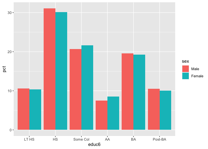
crosstab(df = illinois, x = sex, y = educ6, weight = weight) %>%
  knitr::kable(digits = 0)
| sex | LT HS | HS | Some Col | AA | BA | Post-BA | n |
|---|---|---|---|---|---|---|---|
| Male | 11 | 31 | 21 | 7 | 20 | 11 | 49108796 |
| Female | 10 | 30 | 22 | 9 | 19 | 10 | 53569718 |
library(ggplot2)
crosstab(df = illinois, x = sex, y = educ6, weight = weight, format = "long") %>%
  ggplot(aes(educ6, pct, fill = sex)) +
  geom_bar(stat = "identity", position = "dodge")

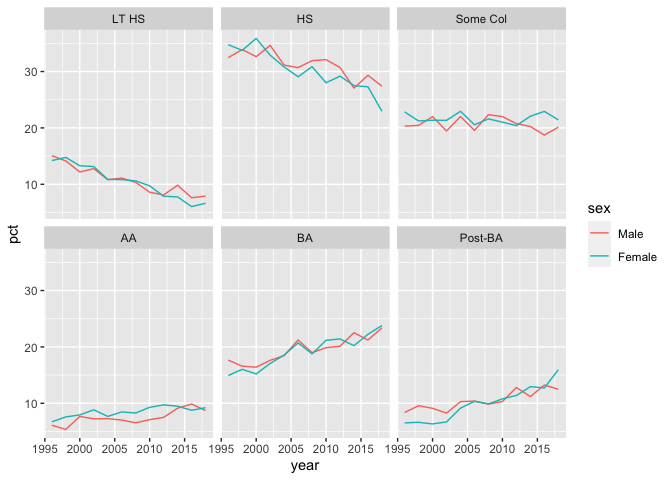
Three-way crosstabs are ideal for plotting time series graphs and/or faceted plots.
crosstab_3way(df = illinois, x = sex, y = educ6, z = year, weight = weight, format = "long") %>%
  ggplot(aes(year, pct, col = sex)) +
  geom_line() +
  facet_wrap(facets = vars(educ6))

Margin of error
Each pollster function comes with a twin function which includes a margin of error column. For example:
moe_topline(df = illinois, variable = voter, weight = weight)
#> # A tibble: 2 x 6
#>   Response  Frequency Percent `Valid Percent`   MOE `Cumulative Percent`
#>   <fct>         <dbl>   <dbl>           <dbl> <dbl>                <dbl>
#> 1 Voted     56230937.    63.7            63.7 0.551                 63.7
#> 2 Not voted 32070164.    36.3            36.3 0.551                100
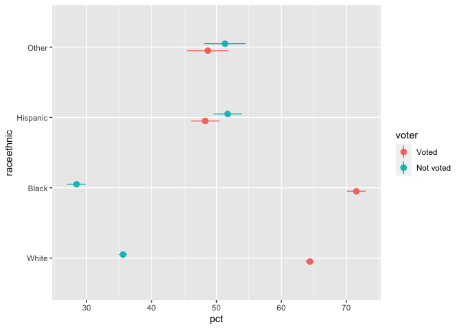
By default, moe_crosstab output comes in long format, but you can also specify wide format.
moe_crosstab(df = illinois, x = raceethnic, y = voter, weight = weight, format = "wide")
#> # A tibble: 4 x 6
#>   raceethnic     n pct_Voted `pct_Not voted` moe_Voted `moe_Not voted`
#>   <fct>      <int>     <dbl>           <dbl>     <dbl>           <dbl>
#> 1 White      24167      64.4            35.6     0.624           0.624
#> 2 Black       3980      71.6            28.4     1.45            1.45
#> 3 Hispanic    2106      48.3            51.7     2.21            2.21
#> 4 Other       1006      48.7            51.3     3.19            3.19
moe_crosstab(df = illinois, x = raceethnic, y = voter, weight = weight) %>%
  ggplot(aes(x = pct, y = raceethnic, xmin = (pct - moe), xmax = (pct + moe), color = voter)) +
  geom_pointrange(position = position_dodge(width = 0.2))

Summary table
summary_table() creates a simple summary table of a weighted numeric variable.
summary_table(df = illinois, variable = age, weight = weight)
#> # A tibble: 1 x 8
#>   variable_name unweighted_obse… weighted_observ… weighted_mean min_value
#>   <chr>                    <int>            <dbl>         <dbl>     <dbl>
#> 1 age                      36207       102678514.          46.2        18
#> # … with 3 more variables: max_value <dbl>, missing_observations <int>,
#> #   missing_weighted_observations <dbl>
You can choose name_style = "pretty" if you want column headings appropriate for a formatted table.
summary_table(df = illinois, variable = age,
              weight = weight, name_style = "pretty") %>%
  knitr::kable()
| Variable | Unweighted obs | Weighted obs | Weighted mean | Min | Max | Unweighted missing | Weighted missing |
|---|---|---|---|---|---|---|---|
| age | 36207 | 102678514 | 46.19646 | 18 | 90 | 0 | 0 |