Sparse and Group Sparse Linear Models.

quadrupen: Sparsity by Worst-Case Quadratic Penalties

Description

Fits the solution paths of classical sparse regression models with efficient active set algorithms by solving small sub-problems. Depending on the penalty, the sub-problems can be solved exactly (i.e. for the LASSO) or with generic solvers. The available optimizer includes quadratic solvers, Newton-based approaches and generic FISTA or PGD algorithms. Also provides a few methods for model selection purpose (information criteria, cross-validation, stability selection).

Quadrupen covers the following regularizers

• LASSO[^1] (Least Absolute Shrinkage and Selection Operator)
• SCAD[^2] (Smoothly Clipped Absolute Deviation)
• MCP[^3] (Minimax Concave Penalty)
• Group-LASSO[^4] ($\ell_1/\ell_2$ or $\ell_1/\ell_\infty$)
• Cooperative-LASSO[^5]
• Sparse Group-LASSO[^6] and Sparse Cooperative-LASSO
• Bounded Regression ($\ell_\infty$-norm).
• LAVA[^7] and the group-LAVA variants for all the group-sparse methods
• Ridge Regression[^8]

For all these regularizers, Quadrupen offers the possibility to add an $\ell_2$/ridge-like “structured” penalty to embed some external knowledge about the statistical dependence between the features. When adding such a penalty to the LASSO, this is sometimes referred to as the “Structured” or “Generalized” Elastic-Net”[^9].

We also provide in the package the implementation of the Generalized Fused-LASSO[^10] originally proposed by Holger Hoefling now archived from CRAN (original repo here).

The original version of Quadrupen only includes Lasso, Elastic-Net and Bounded regression. It was used as an illustration for our paper “Sparsity by worst-case penalties”[^11]. I eventually used it to include my personal implementation of sparse methods for linear regression.

While likely not as fast as highly specialized packages like glmnet, the use of a working set algorithm combined with efficient solvers, sparse matrix support when applicable, and templated C++ code makes it both competitive and versatile.

Installation

devtools::install_github("jchiquet/quadrupen")

A couple of vignettes introduce the basics and more advanced uses of the functions and classes implemented in the package. Other examples can be found in the documentation and in the inst directory. Here is a more illustrative one:

Example: structured penalized regression

This example is extracted from chapter 1 of my habilitation. You can get more insight by reading pages 65-66, 70-71.

First, load the package

library(quadrupen)

'quadrupen' package version 1.0-0

A toy data set advocating for structured regularization

See pages 29–30 in my habilitation. Code for additional functions is given at the end of the present document (Appendix).

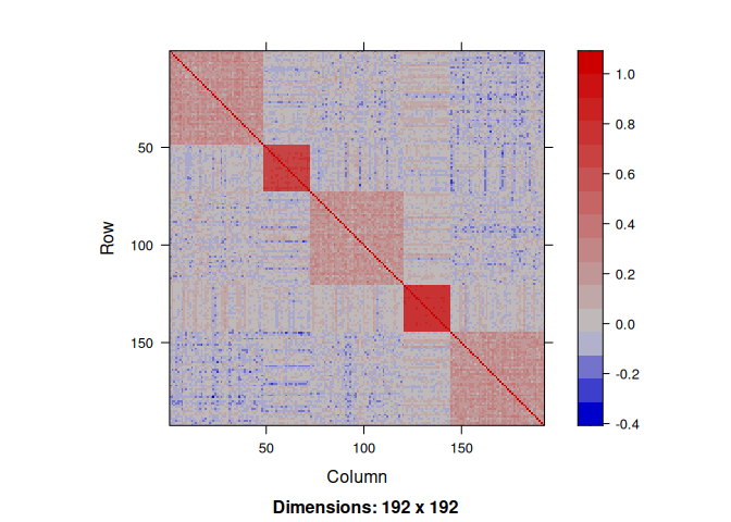
We draw data from a linear regression where the regression parameters are defined group-wise. The regressors are correlated according to the same block pattern.

n <- 200
p <- 192

## model settings: block wise
mu <- 0
group <- c(p/4,p/8,p/4,p/8,p/4)
labels <- factor(rep(paste("group", 1:5), group))
beta   <- rep(c(0.25,1,-0.25,-1,0.25), group)
x <- rPred.block(n, p, sizes = group, rho=c(0.25, 0.75, 0.25, 0.75, 0.25))

Indeed, the correlation structure between the regressors exhibits a strong pattern:

We draw the response variable by fixing the variance of the noise ratio to get an $R^2$ equal to $0.8$.

dat <- rlm(x,beta,mu,r2=0.8)
y <- dat$y
sigma <- dat$sigma

Regularization without prior knowledge

Now we try the available penalized regression methods in quadrupen to fit the regularization path to this data set

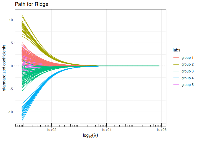
Ridge regression ($\ell_2$ penalty)

plot(ridge(x,y, intercept=FALSE), labels=labels)

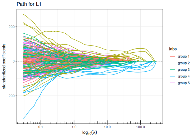
Lasso ($\ell_1$ penalty)

plot(lasso(x,y, intercept=FALSE), labels=labels)

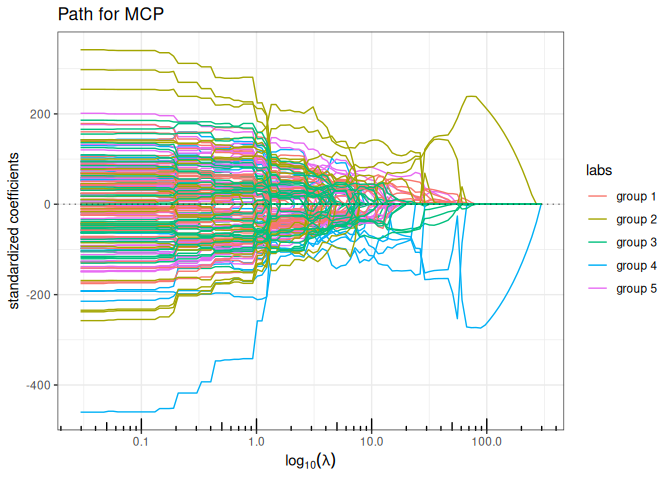
MCP (Minimax Concave Penalty)

plot(mcp(x,y, intercept=FALSE), labels=labels)

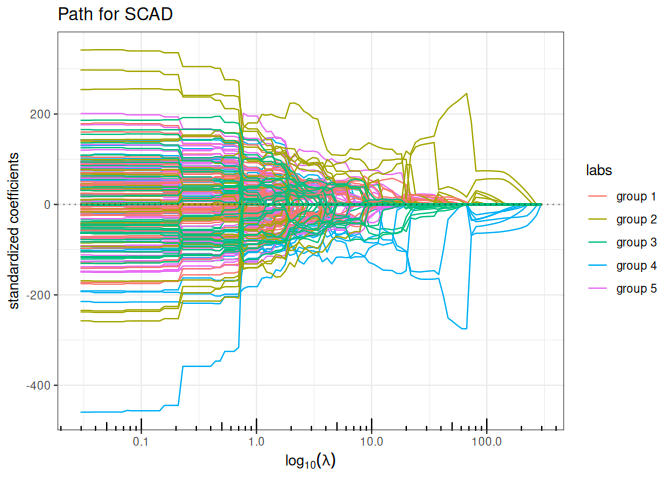
SCAD (Smoothly Clipped Absolute Deviation)

plot(scad(x,y, intercept=FALSE), labels=labels)

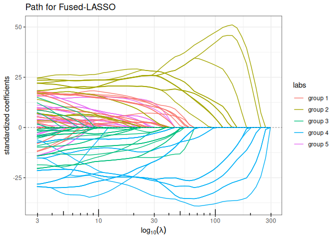
Fused-LASSO (contiguity penalty)

plot(fused_lasso(x,y, lambda2 = 5, intercept=FALSE), labels=labels)

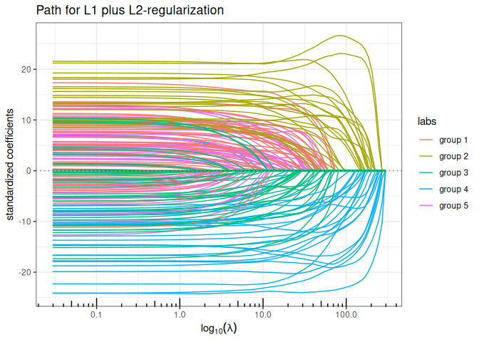
Elastic-net ($\ell_1+\ell_2$ penalty)

plot(elastic_net(x,y, lambda2=1, intercept=FALSE), labels=labels)

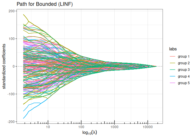
Bounded regression ($\ell_\infty$ penalty)

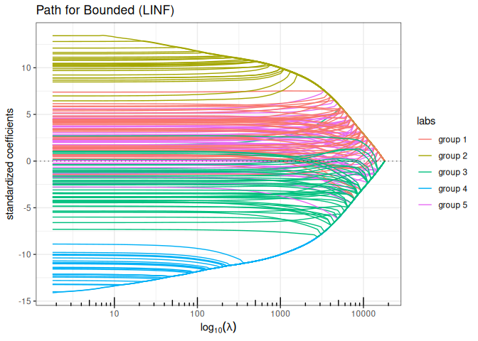
plot(bounded_reg(x,y, lambda2=0, intercept=FALSE), labels=labels)

Bounded regression + Ridge ($\ell_\infty+\ell_2$ penalty)

plot(bounded_reg(x,y, lambda2=5, intercept=FALSE), labels=labels)

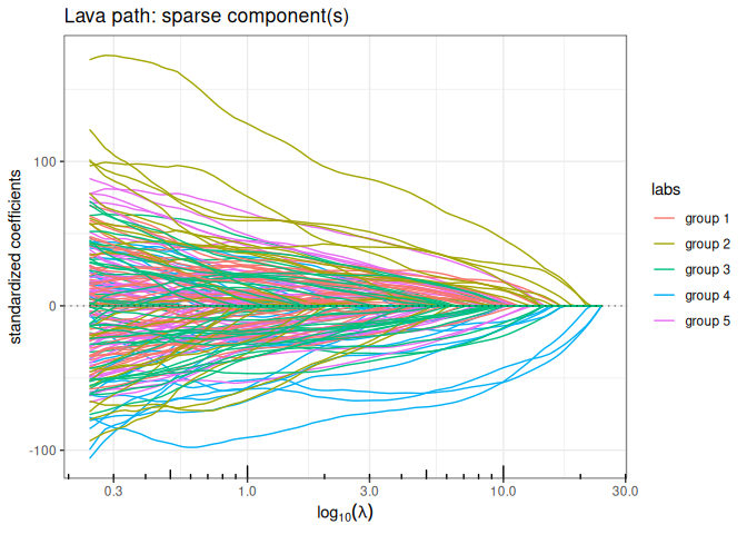
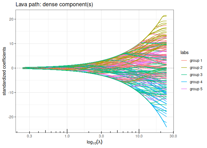
Lava (sparse + dense signal decomposition)

out_lava <- lava(x,y, lambda2=1, intercept=FALSE)
out_lava$plot_path(component = "sparse", labels=labels)

out_lava$plot_path(component = "dense", labels=labels)

Regularization with smooth prior knowledge

Now let’s define the graph associated with the groups of the regressor and compute the Graph Laplacian. We add a small value on the diagonal to ensure strict positive definiteness (in the future, this matrix should preferentially be defined with a graph).

A <- Matrix::bdiag(lapply(group, function(s) matrix(1,s,s))) ; diag(A) <- 0
L <- -A; diag(L) <- Matrix::colSums(A) + 1e-2

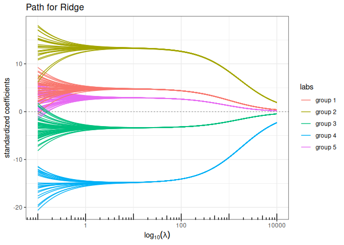
Now, we run all the methods having a ridge-like regularization by replacing the ridge penalty $| \cdot |2^2$ with $| \cdot |{\mathbf{L}}^2$ to enforce some structure in the regularization: the solution paths look a lot more convincing.

Structured/Generalized Ridge regression ($\ell_2$ penalty)

plot(ridge(x,y, lambda = 10^seq(4,-1,len=100), struct = L, intercept=FALSE), labels=labels)

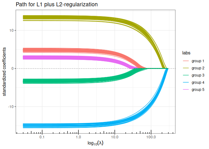
Structured/Generalized Elastic-net ($\ell_1+\ell_2$ penalty)

plot(elastic_net(x,y, struct = L, lambda2=1, intercept=FALSE), labels=labels)

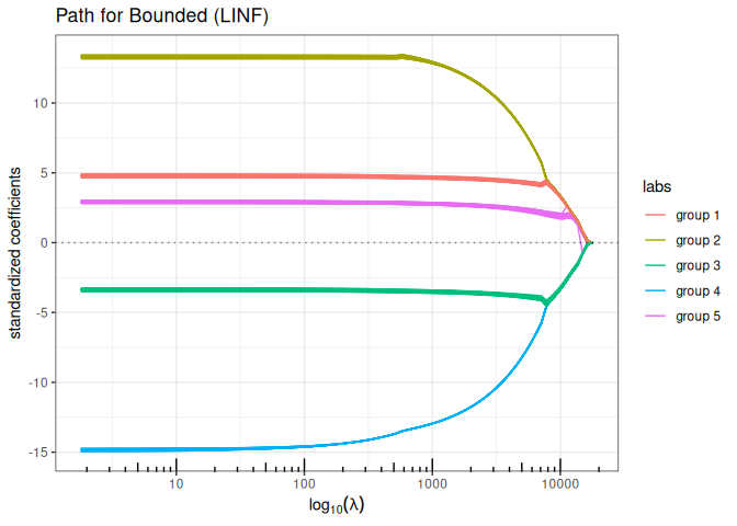
Bounded regression + structured/Generalized Ridge ($\ell_\infty+\ell_2$ penalty)

plot(bounded_reg(x,y, struct = L, lambda2=5, intercept=FALSE), labels=labels)

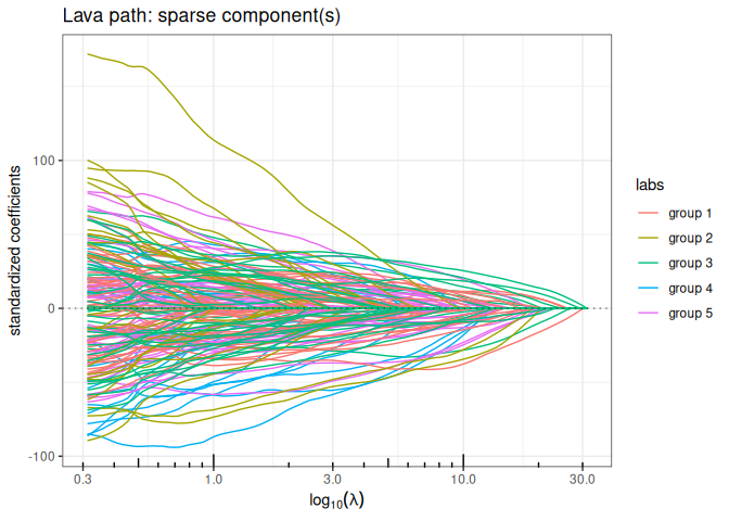
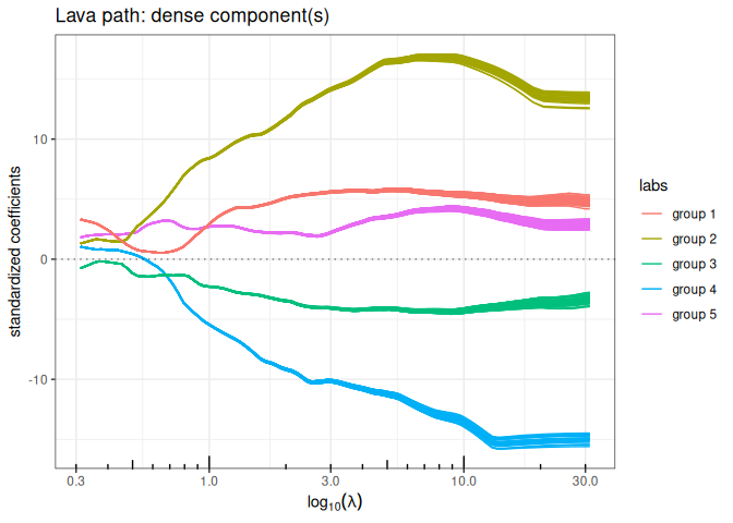
Lava (sparse + structured dense)

out_lava <- lava(x,y, lambda2=1, struct = L, intercept=FALSE)
out_lava$plot_path(component = "sparse", labels=labels)

out_lava$plot_path(component = "dense", labels=labels)

Regularization with hard prior knowledge

We can use the correlation structure as a proxy for forming groups of variables, and use group-sparse regularization. We offer three variants of group sparse regularization in quadrupen: standard group-lasso ($\ell_1/\ell_2$ mixed norm), type 2 group Lasso ($\ell_1/\ell_\infty$ mixed norm) and the cooperative-lasso, an original proposition.

We first define a group index vector to encode the group memberships:

group <- rep(1:length(group), group)

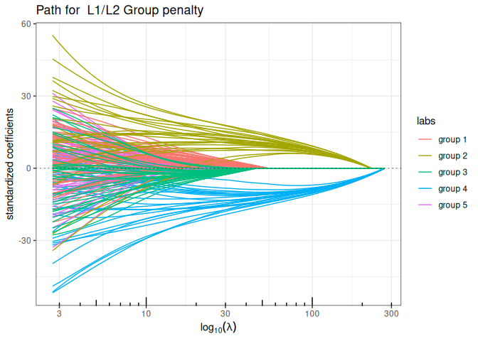
Group Lasso (group sparse L1/L2)

plot(group_lasso(x, y, group, intercept=FALSE), labels=labels)

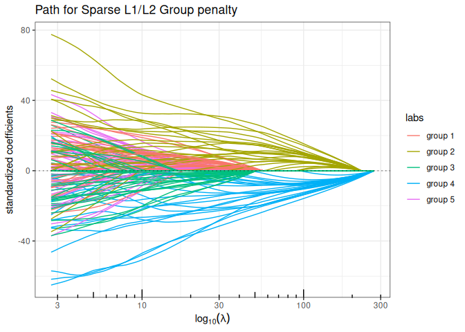
Sparse Group Lasso (mixing L1 + group sparse L1/L2)

plot(sparse_group_lasso(x, y, group, alpha = 0.75, intercept=FALSE), labels=labels)

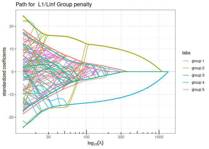
Group-Lasso (group sparse L1/LInf)

plot(group_l1linf(x, y, group, intercept=FALSE), labels=labels)

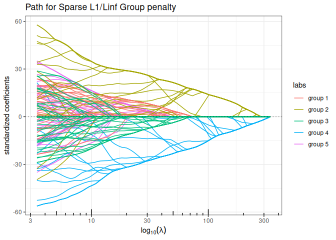
Sparse Group Lasso (mixing L1 + group sparse L1/LInf)

plot(sparse_group_l1linf(x, y, group, alpha = 0.75, intercept=FALSE), labels=labels)

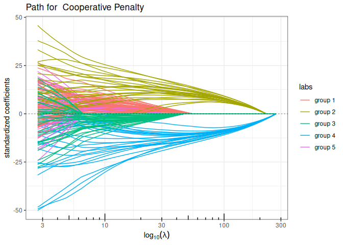
Cooperative-Lasso (sign-coherent group lasso)

plot(coop_lasso(x, y, group, intercept=FALSE), labels=labels)

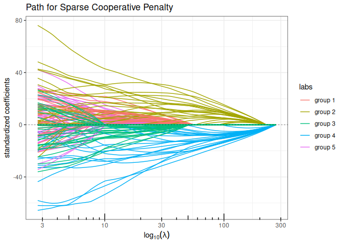
Sparse Cooperative Lasso (mixing L1 + Cooperative norm)

plot(sparse_coop_lasso(x, y, group, alpha = 0.75, intercept=FALSE), labels=labels)

Regularization mixing smooth and hard prior knowledge

We allow the possibility to add a structured-$\ell_2$ penalty to these mixed-group penalties, in order to introduce additional smoothing prior in the regularization, just like in the structured version of the Elastic-Net and Ridge regression. For this, the function group_sparse_lm is the most generic group-wise function, which generalizes all the above models by allowing the addition of an $\ell_2$-structured penalty.

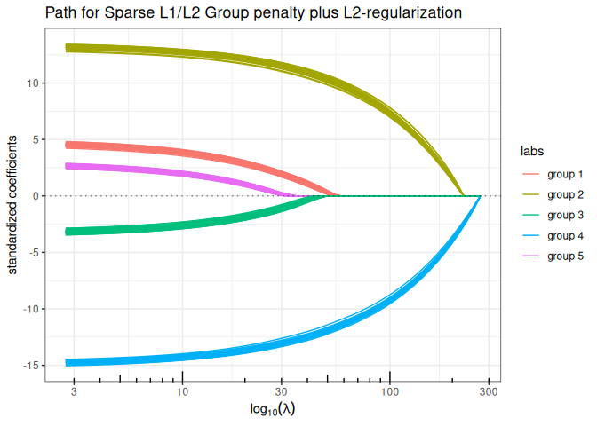
Sparse Group-Lasso L2 + Structured ElasticNet (group sparse L1/L2 + structured L2)

plot(group_sparse_lm(x, y, group, type = "l2", alpha = 0.5, lambda2 = 2, struct = L, intercept=FALSE), labels=labels)

[!NOTE]

Disclaimer about the use of AI

I wrote all the R and C++ code, which is a collection of various pieces accumulated over the years (except for the Fused-Lasso code, which was written by Holger Hoefling). I recently put all these pieces together. I used Claude code to help me refactor and optimise certain parts of the C++ code, as well as to review and generate parts of the documentation.

Appendix: functions for data generation

chol.uniform <- function(p,rho) {

  q <- 0     ## sum_k^(i-1) c.k^2
  cii <- 1   ## current value of the diagonal
  c.i <- rho ## current value of the off-diagonal term
  Cii <- cii ## vector of diagonal terms
  C.i <- c.i ## vector of off-diagonal terms
  for (i in 2:p) {
    q <- q + c.i^2
    cii <- sqrt(1-q)
    c.i <- (rho-q)/cii
    Cii <- c(Cii,cii)
    C.i <- c(C.i,c.i)
  }
  return(list(cii=Cii, c.i=C.i[-p]))
}

rlm <- function(x,beta,mu=0,r2=NULL,sigma=1) {
  n <- nrow(x)
  if (!is.null(r2))
      sigma  <- as.numeric(sqrt((1-r2)/r2 * t(beta) %*% cov(x) %*% beta))
  epsilon <- rnorm(n) * sigma
  y <- mu + x %*% beta + epsilon
  r2 <- 1 - sum(epsilon^2) / sum((y-mean(y))^2)
  return(list(y=y,sigma=sigma))
}

## Blockwise structure
## the length of rho determine the number of blocs
## each group must be > 1 individual
rPred.block <- function(n, p, sizes=rmultinom(1,p,rep(p/K,K)), rho=rep(0.75,4)) {

  K <- length(rho)
  stopifnot(sum(sizes) == p | length(rho) != length(sizes))
  Cs <- lapply(1:K, function(k) chol.uniform(sizes[k],rho[k]))

  rmv <- function() {
      return(
      unlist(lapply(1:K, function(k) {
        z <- rnorm(sizes[k])
        Cs[[k]]$cii*z + c(0,cumsum(z[-sizes[k]]*Cs[[k]]$c.i))
      }))
      )
  }
  return(t(replicate(n, rmv(), simplify=TRUE)))
}

References

[^1]: Tibshirani, Robert. “Regression shrinkage and selection via the lasso.” Journal of the Royal Statistical Society Series B: Statistical Methodology 58.1 (1996): 267-288.

[^2]: Fan, Jianqing, and Runze Li. “Variable selection via nonconcave penalized likelihood and its oracle properties.” Journal of the American statistical Association 96.456 (2001): 1348-1360.

[^3]: Zhang, C. H. Nearly unbiased variable selection under minimax concave penalty. The Annals of Statistics, 38(2), (2010): 894-942.

[^4]: Yuan, Ming, and Yi Lin. “Model selection and estimation in regression with grouped variables.” Journal of the Royal Statistical Society Series B: Statistical Methodology 68.1 (2006): 49-67.

[^5]: Chiquet, Julien, Yves Grandvalet, and Camille Charbonnier. “Sparsity with sign-coherent groups of variables via the cooperative-lasso.” (2012): 795-830.

[^6]: Simon, Noah, et al. “A sparse-group lasso.” Journal of computational and graphical statistics 22.2 (2013): 231-245.

[^7]: Chernozhukov, Victor, Christian Hansen, and Yuan Liao. “A lava attack on the recovery of sums of dense and sparse signals.” The Annals of Statistics (2017): 39-76.

[^8]: Hoerl, Arthur E., and Robert W. Kennard. “Ridge regression: Biased estimation for nonorthogonal problems.” Technometrics 12.1 (1970): 55-67.

[^9]: Slawski, Martin. “The structured elastic net for quantile regression and support vector classification.” Statistics and Computing 22.1 (2012): 153-168.

[^10]: Hoefling, Holger. “A path algorithm for the fused lasso signal approximator.” Journal of Computational and Graphical Statistics 19.4 (2010): 984-1006.

[^11]: Grandvalet, Yves, Julien Chiquet, and Christophe Ambroise. “Sparsity by worst-case penalties.” arXiv preprint arXiv:1210.2077 (2012).