Description

Compiler for R.

Description

Compiles R functions annotated with type and shape declarations to provide extremely fast performance and robust runtime type checking. Supports both just-in-time (JIT) and ahead-of-time (AOT) compilation. Compilation is performed by lowering R code to Fortran.

README.md

cran.r-project.org

quickr

The goal of quickr is to make your R code run quicker.

Overview

R is an extremely flexible and dynamic language, but that flexibility and dynamicism can come at the expense of speed. This package lets you trade back some of that flexibility for some speed, for the context of a single function.

The main exported function is quick(), here is how you use it.

library(quickr)

convolve <- quick(function(a, b) {
  declare(type(a = double(NA)),
          type(b = double(NA)))
  ab <- double(length(a) + length(b) - 1)
  for (i in seq_along(a)) {
    for (j in seq_along(b)) {
      ab[i+j-1] <- ab[i+j-1] + a[i] * b[j]
    }
  }
  ab
})

quick() returns a quicker R function. How much quicker? Let’s benchmark it! For reference, we’ll also compare it to a pure-C implementation.

slow_convolve <- function(a, b) {
  declare(type(a = double(NA)),
          type(b = double(NA)))
  ab <- double(length(a) + length(b) - 1)
  for (i in seq_along(a)) {
    for (j in seq_along(b)) {
      ab[i+j-1] <- ab[i+j-1] + a[i] * b[j]
    }
  }
  ab
}

library(quickr)
quick_convolve <- quick(slow_convolve)

convolve_c <- inline::cfunction(
  sig = c(a = "SEXP", b = "SEXP"), body = r"({
    int na, nb, nab;
    double *xa, *xb, *xab;
    SEXP ab;

    a = PROTECT(Rf_coerceVector(a, REALSXP));
    b = PROTECT(Rf_coerceVector(b, REALSXP));
    na = Rf_length(a); nb = Rf_length(b); nab = na + nb - 1;
    ab = PROTECT(Rf_allocVector(REALSXP, nab));
    xa = REAL(a); xb = REAL(b); xab = REAL(ab);
    for(int i = 0; i < nab; i++) xab[i] = 0.0;
    for(int i = 0; i < na; i++)
        for(int j = 0; j < nb; j++)
            xab[i + j] += xa[i] * xb[j];
    UNPROTECT(3);
    return ab;
})")



a <- runif (100000); b <- runif (100)

timings <- bench::mark(
  r = slow_convolve(a, b),
  quickr = quick_convolve(a, b),
  c = convolve_c(a, b),
  min_time = 2
)
timings
#> # A tibble: 3 × 6
#>   expression      min   median `itr/sec` mem_alloc `gc/sec`
#>   <bch:expr> <bch:tm> <bch:tm>     <dbl> <bch:byt>    <dbl>
#> 1 r             1.05s    1.05s     0.955     847KB    0.955
#> 2 quickr        4.8ms   5.09ms   195.        782KB    3.07 
#> 3 c            4.73ms   5.04ms   196.        782KB    3.09
plot(timings) + bench::scale_x_bench_time(base = NULL)

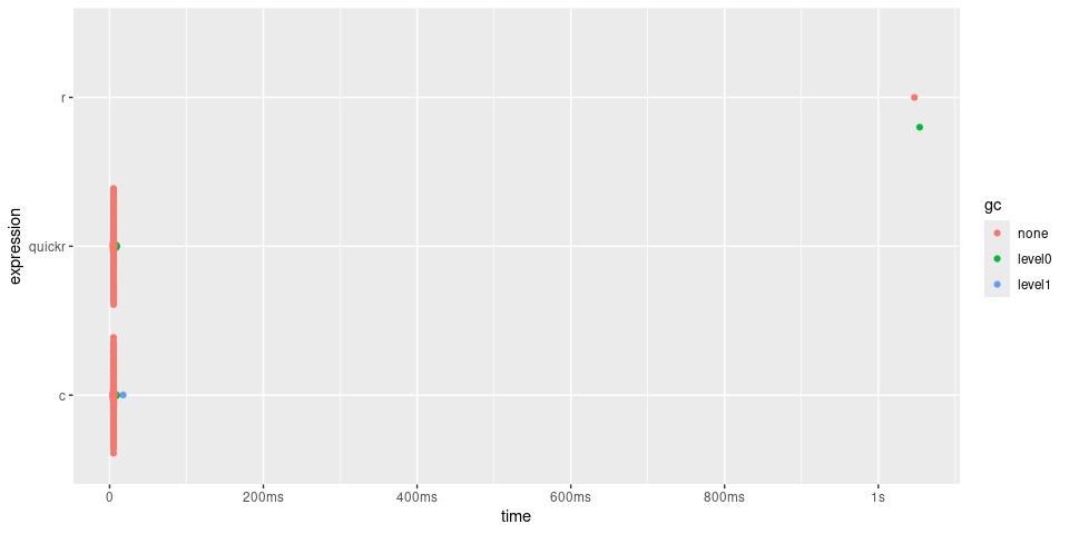
In the case of convolve(), quick() returns a function approximately 200 times quicker, giving similar performance to the C function.

quick() can accelerate any R function, with some restrictions:

Function arguments must have their types and shapes declared using declare().
Only atomic vectors, matrices, and array are currently supported: integer, double, logical, and complex.
The return value must be an atomic array (e.g., not a list)
Named variables must have consistent shapes throughout their lifetimes.
NA values are not supported.
Only a subset of R’s vocabulary is currently supported.

#>  [1] -         :         !=        (         [         [<-       {        
#>  [8] *         /         &         &&        %/%       %%        ^        
#> [15] +         <         <-        <=        =         ==        >        
#> [22] >=        |         ||        Arg       Conj      Fortran   Im       
#> [29] Mod       Re        abs       acos      asin      atan      c        
#> [36] cat       cbind     ceiling   character cos       declare   double   
#> [43] exp       floor     for       if        ifelse    integer   length   
#> [50] log       log10     logical   matrix    max       min       numeric  
#> [57] print     prod      raw       seq       sin       sqrt      sum      
#> [64] tan       which.max which.min

Many of these restrictions are expected to be relaxed as the project matures. However, quickr is intended primarily for high-performance numerical computing, so features like polymorphic dispatch or support for complex or dynamic types are out of scope.

`declare(type())` syntax:

The shape and mode of all function arguments must be declared. Local and return variables may optionally also be declared.

declare(type()) also has support for declaring size constraints, or size relationships between variables. Here are some examples of declare calls:

declare(type(x = double(NA))) # x is a 1-d double vector of any length
declare(type(x = double(10))) # x is a 1-d double vector of length 10
declare(type(x = double(1)))  # x is a scalar double

declare(type(x = integer(2, 3)))  # x is a 2-d integer matrix with dim (2, 3)
declare(type(x = integer(NA, 3))) # x is a 2-d integer matrix with dim (<any>, 3)

# x is a 4-d logical matrix with dim (<any>, 24, 24, 3)
declare(type(x = logical(NA, 24, 24, 3)))

# x and y are 1-d double vectors of any length
declare(type(x = double(NA)),
        type(y = double(NA)))

# x and y are 1-d double vectors of the same length
declare(
  type(x = double(n)),
  type(y = double(n)),
)

# x and y are 1-d double vectors, where length(y) == length(x) + 2
declare(type(x = double(n)),
        type(y = double(n+2)))

More examples:

`viterbi`

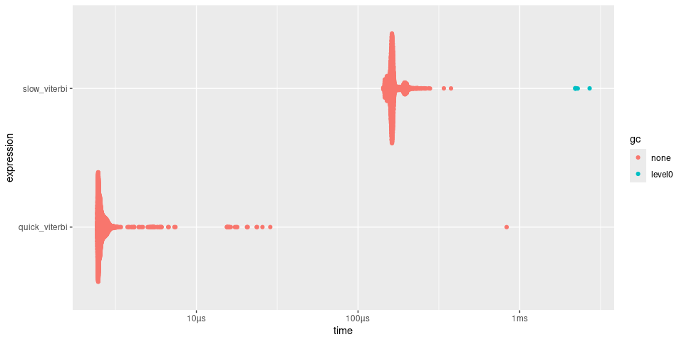
The Viterbi algorithm is an example of a dynamic programming algorithm within the family of Hidden Markov Models (https://en.wikipedia.org/wiki/Viterbi_algorithm). Here, quick() makes the viterbi() approximately 50 times faster.

slow_viterbi <- function(observations, states, initial_probs, transition_probs, emission_probs) {
    declare(
      type(observations = integer(num_steps)),
      type(states = integer(num_states)),
      type(initial_probs = double(num_states)),
      type(transition_probs = double(num_states, num_states)),
      type(emission_probs = double(num_states, num_obs)),
    )

    trellis <- matrix(0, nrow = length(states), ncol = length(observations))
    backpointer <- matrix(0L, nrow = length(states), ncol = length(observations))
    trellis[, 1] <- initial_probs * emission_probs[, observations[1]]

    for (step in 2:length(observations)) {
      for (current_state in 1:length(states)) {
        probabilities <- trellis[, step - 1] * transition_probs[, current_state]
        trellis[current_state, step] <- max(probabilities) * emission_probs[current_state, observations[step]]
        backpointer[current_state, step] <- which.max(probabilities)
      }
    }

    path <- integer(length(observations))
    path[length(observations)] <- which.max(trellis[, length(observations)])
    for (step in seq(length(observations) - 1, 1)) {
      path[step] <- backpointer[path[step + 1], step + 1]
    }

    out <- states[path]
    out
}

quick_viterbi <- quick(slow_viterbi)

set.seed(1234)
num_steps <- 16
num_states <- 8
num_obs <- 16

observations <- sample(1:num_obs, num_steps, replace = TRUE)
states <- 1:num_states
initial_probs <- runif (num_states)
initial_probs <- initial_probs / sum(initial_probs)  # normalize to sum to 1
transition_probs <- matrix(runif (num_states * num_states), nrow = num_states)
transition_probs <- transition_probs / rowSums(transition_probs)  # normalize rows
emission_probs <- matrix(runif (num_states * num_obs), nrow = num_states)
emission_probs <- emission_probs / rowSums(emission_probs)  # normalize rows

timings <- bench::mark(
  slow_viterbi = slow_viterbi(observations, states, initial_probs,
                              transition_probs, emission_probs),
  quick_viterbi = quick_viterbi(observations, states, initial_probs,
                                transition_probs, emission_probs)
)
timings
#> # A tibble: 2 × 6
#>   expression         min   median `itr/sec` mem_alloc `gc/sec`
#>   <bch:expr>    <bch:tm> <bch:tm>     <dbl> <bch:byt>    <dbl>
#> 1 slow_viterbi  143.04µs    162µs     6047.     178KB     14.5
#> 2 quick_viterbi   2.43µs   2.53µs   368609.        0B      0
plot(timings)

Diffusion simulation

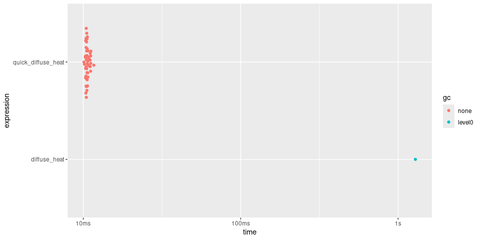
Simulate how heat spreads over time across a 2D grid, using the finite difference method applied to the Heat Equation.

Here, quick() returns a function over 100 time faster.

diffuse_heat <- function(nx, ny, dx, dy, dt, k, steps) {
  declare(
    type(nx = integer(1)),
    type(ny = integer(1)),
    type(dx = integer(1)),
    type(dy = integer(1)),
    type(dt = double(1)),
    type(k = double(1)),
    type(steps = integer(1))
  )

  # Initialize temperature grid
  temp <- matrix(0, nx, ny)
  temp[nx / 2, ny / 2] <- 100  # Initial heat source in the center

  # Time stepping
  for (step in seq_len(steps)) {
    # Apply boundary conditions
    temp[1, ] <- 0
    temp[nx, ] <- 0
    temp[, 1] <- 0
    temp[, ny] <- 0

    # Update using finite differences
    temp_new <- temp
    for (i in 2:(nx - 1)) {
      for (j in 2:(ny - 1)) {
        temp_new[i, j] <- temp[i, j] + k * dt *
          ((temp[i + 1, j] - 2 * temp[i, j] + temp[i - 1, j]) /
             dx ^ 2 + (temp[i, j + 1] - 2 * temp[i, j] + temp[i, j - 1]) / dy ^ 2)
      }
    }
    temp <- temp_new

  }

  temp
}

quick_diffuse_heat <- quick(diffuse_heat)

# Parameters
nx <- 100L      # Grid size in x
ny <- 100L      # Grid size in y
dx <- 1L        # Grid spacing
dy <- 1L        # Grid spacing
dt <- 0.01      # Time step
k <- 0.1        # Thermal diffusivity
steps <- 500L   # Number of time steps

timings <- bench::mark(
  diffuse_heat = diffuse_heat(nx, ny, dx, dy, dt, k, steps),
  quick_diffuse_heat = quick_diffuse_heat(nx, ny, dx, dy, dt, k, steps)
)
#> Warning: Some expressions had a GC in every iteration; so filtering is
#> disabled.
summary(timings, relative = TRUE)
#> Warning: Some expressions had a GC in every iteration; so filtering is
#> disabled.
#> # A tibble: 2 × 6
#>   expression           min median `itr/sec` mem_alloc `gc/sec`
#>   <bch:expr>         <dbl>  <dbl>     <dbl>     <dbl>    <dbl>
#> 1 diffuse_heat        127.   122.        1      1014.      Inf
#> 2 quick_diffuse_heat    1      1       121.        1       NaN
plot(timings)

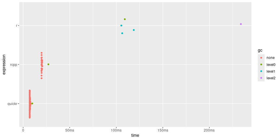
Rolling Mean

Here is quickr used to calculate a rolling mean. Note that the CRAN package RcppRoll already provides a highly optimized rolling mean, which we include in the benchmarks for comparison.

slow_roll_mean <- function(x, weights, normalize = TRUE) {
  declare(
    type(x = double(NA)),
    type(weights = double(NA)),
    type(normalize = logical(1))
  )
  out <- double(length(x) - length(weights) + 1)
  n <- length(weights)
  if (normalize)
    weights <- weights/sum(weights)*length(weights)

  for(i in seq_along(out)) {
    out[i] <- sum(x[i:(i+n-1)] * weights) / length(weights)
  }
  out
}

quick_roll_mean <- quick(slow_roll_mean)

x <- dnorm(seq(-3, 3, len = 100000))
weights <- dnorm(seq(-1, 1, len = 100))

timings <- bench::mark(
  r = slow_roll_mean(x, weights),
  rcpp = RcppRoll::roll_mean(x, weights = weights),
  quickr = quick_roll_mean(x, weights = weights)
)
#> Warning: Some expressions had a GC in every iteration; so filtering is
#> disabled.
timings
#> # A tibble: 3 × 6
#>   expression      min   median `itr/sec` mem_alloc `gc/sec`
#>   <bch:expr> <bch:tm> <bch:tm>     <dbl> <bch:byt>    <dbl>
#> 1 r           105.4ms 109.13ms      7.42  124.31MB    22.3 
#> 2 rcpp         19.7ms  19.84ms     49.4     4.44MB     1.98
#> 3 quickr          7ms   7.09ms    138.    781.35KB     2.00

timings$expression <- factor(names(timings$expression), rev(names(timings$expression)))
plot(timings) + bench::scale_x_bench_time(base = NULL)

Using `quickr` in an R package

When called in a package, quick() will pre-compile the quick functions and place them in the ./src directory. Run devtools::load_all() or quickr::compile_package() to ensure that the generated files in ./src and ./R are in sync with each other.

Installation

You can install quickr from CRAN with:

install.packages("quickr")

You can install the development version of quickr from GitHub with:

# install.packages("pak")
pak::pak("t-kalinowski/quickr")

You will also need a C and Fortran compiler, preferably the same ones used to build R itself.

On macOS:

Make sure xcode tools and gfortran are installed, as described in https://mac.r-project.org/tools/. In Terminal, run:

sudo xcode-select --install
# curl -LO https://mac.r-project.org/tools/gfortran-12.2-universal.pkg # R 4.4
curl -LO https://mac.r-project.org/tools/gfortran-14.2-universal.pkg   # R 4.5
sudo installer -pkg gfortran-12.2-universal.pkg -target /

On Windows:

Install the latest version of Rtools

On Linux:

The “Install Required Dependencies” section here provides detailed instructions for installing R build tools on various Linux flavors.

r-quickr

quickr

Overview

`declare(type())` syntax:

More examples:

`viterbi`

Diffusion simulation

Rolling Mean

Using `quickr` in an R package

Installation

Version

License

Status

Source

Homepage

Platforms (75)

quickr

Overview

declare(type()) syntax:

More examples:

viterbi

Diffusion simulation

Rolling Mean

Using quickr in an R package

Installation

Version

License

Status

Source

Homepage

Platforms75 (75)

`declare(type())` syntax:

`viterbi`

Using `quickr` in an R package

Platforms (75)