AdaBoost Framework for Any Classifier.
Introduction
This package aims to enable the use of classifiers in boosting family algorithms, apart from decision trees and other classical weak classifiers. The current scope of the package includes Real AdaBoost and Discrete AdaBoost, as well as multiclass versions of these methods, the SAMME and SAMME.R algorithms.
Future plans
I am aware that there have been attempts to create frameworks that allow using custom functions in boosting (e.g. boostr). However, they are too complex to my taste. I haven’t seen a simple-to-use package that handles different boosting methods. What can be done simply in Python, why can’t it be done in R? That is my point. The package is still in the starting phase (a baby package). Things on my mind:
- I will add more boosting algorithms such as GentleBoost, LogitBoost, Gradient Boosting and XGBoost.
- I will enable the establishment of not only classification but also regression models with these methods.
- In accordance with the main purpose of the package, I will allow the use of regression models prepared by the user in boosting algorithms.
- Custom resampling methods to use in each boosting step for class imbalanced datasets and some pre-ready methods such as random-undersampling, random-oversampling and SMOTE.
- Data pre-processing methods (e.g. PCA, KPCA, discretization, dummyfication).
- Missing data handling methods (e.g. list-wise deletion, row-wise deletion, data imputation)
- If I can, I will add a generalizable feature importance function for all weak classifier (or regression) methods. I’m not sure it can be done. I will work on this issue. I am open to any advice on this matter.
- I will prepare a shiny app inside the package, which you can upload your own data and use any functions available. Varying visualizations and performance metrics will be available. And you will be able to add your custom function using the app.
- I can add the bagging algorithms after all the plans are complete. But I can’t say I’m very keen on this, since it is just model averaging with bootstrapped models. I am not a fan of bagging.
booster function
There is a function for each method in the package. But the main function is the booster. By using this function it will be possible to access everything. Let me give you information about the features of this function and how to use it. First of all, 2 different AdaBoost methods can be applied with the booster function: Real AdaBoost and Discrete AdaBoost. Let us use glass0 dataset in imbalance package and prepare a train and test dataset. test dataset is not mandatory.
library(rbooster)
cv_sampler <- function(y, train_proportion) {
  unlist(lapply(unique(y), function(m) sample(which(y==m), round(sum(y==m))*train_proportion)))
}

library(imbalance)
data <- glass0
p <- ncol(data) - 1

x <- data[,1:p]
y <- data[, p + 1]

train_i <- cv_sampler(y, 0.9)
x_train <- x[train_i,]
y_train <- y[train_i]

x_test <- x[-train_i,]
y_test <- y[-train_i]
This is a two-class dataset. Let us use decision tree to build Discrete and Real AdaBoost models.
m_discrete <- booster(x_train = x_train,
        y_train = y_train,
        classifier = "rpart",
        method = "discrete",
        x_test = x_test,
        y_test = y_test,
        weighted_bootstrap = FALSE,
        max_iter = 20,
        lambda = 1,
        print_detail = TRUE,
        print_plot = TRUE,
        bag_frac = 0.8,
        p_weak = 4)
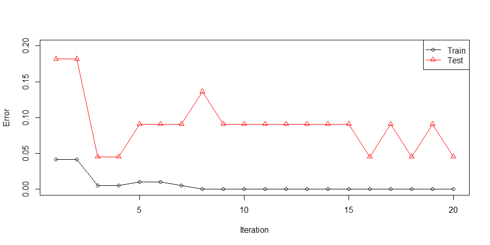
#> 1 Train err:0.04167, Test err:0.18182, Weighted err:0.04167
#> 2 Train err:0.04167, Test err:0.18182, Weighted err:0.07195
#> 3 Train err:0.00521, Test err:0.04545, Weighted err:0.04014
#> 4 Train err:0.00521, Test err:0.04545, Weighted err:0.11524
#> 5 Train err:0.01042, Test err:0.09091, Weighted err:0.07580
#> 6 Train err:0.01042, Test err:0.09091, Weighted err:0.13923
#> 7 Train err:0.00521, Test err:0.09091, Weighted err:0.08863
#> 8 Train err:0.00000, Test err:0.13636, Weighted err:0.05526
#> 9 Train err:0.00000, Test err:0.09091, Weighted err:0.06539
#> 10 Train err:0.00000, Test err:0.09091, Weighted err:0.18110
#> 11 Train err:0.00000, Test err:0.09091, Weighted err:0.12768
#> 12 Train err:0.00000, Test err:0.09091, Weighted err:0.24721
#> 13 Train err:0.00000, Test err:0.09091, Weighted err:0.06630
#> 14 Train err:0.00000, Test err:0.09091, Weighted err:0.10293
#> 15 Train err:0.00000, Test err:0.09091, Weighted err:0.07404
#> 16 Train err:0.00000, Test err:0.04545, Weighted err:0.08221
#> 17 Train err:0.00000, Test err:0.09091, Weighted err:0.12928
#> 18 Train err:0.00000, Test err:0.04545, Weighted err:0.14301
#> 19 Train err:0.00000, Test err:0.09091, Weighted err:0.13722
#> 20 Train err:0.00000, Test err:0.04545, Weighted err:0.08173
m_real <- booster(x_train = x_train,
                      y_train = y_train,
                      classifier = "rpart",
                      method = "real",
                      x_test = x_test,
                      y_test = y_test,
                      weighted_bootstrap = FALSE,
                      max_iter = 20,
                      lambda = 1,
                      print_detail = TRUE,
                      print_plot = TRUE,
                      bag_frac = 0.8,
                      p_weak = 4)
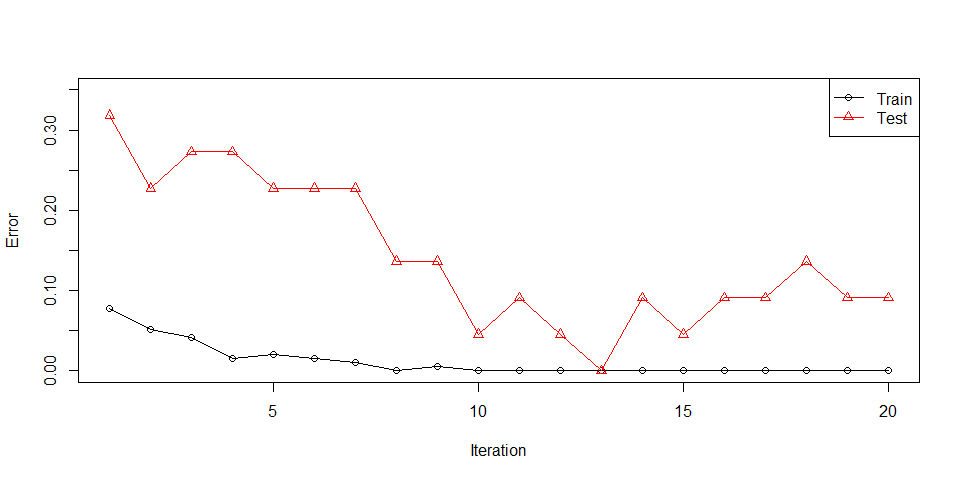
#> 1 Train err:0.07812, Test err:0.31818, Weighted err:0.07812
#> 2 Train err:0.05208, Test err:0.22727, Weighted err:0.01914
#> 3 Train err:0.04167, Test err:0.27273, Weighted err:0.07696
#> 4 Train err:0.01562, Test err:0.27273, Weighted err:0.26836
#> 5 Train err:0.02083, Test err:0.22727, Weighted err:0.02338
#> 6 Train err:0.01562, Test err:0.22727, Weighted err:0.46096
#> 7 Train err:0.01042, Test err:0.22727, Weighted err:0.02315
#> 8 Train err:0.00000, Test err:0.13636, Weighted err:0.02416
#> 9 Train err:0.00521, Test err:0.13636, Weighted err:0.13217
#> 10 Train err:0.00000, Test err:0.04545, Weighted err:0.10323
#> 11 Train err:0.00000, Test err:0.09091, Weighted err:0.05400
#> 12 Train err:0.00000, Test err:0.04545, Weighted err:0.12940
#> 13 Train err:0.00000, Test err:0.00000, Weighted err:0.07897
#> 14 Train err:0.00000, Test err:0.09091, Weighted err:0.09409
#> 15 Train err:0.00000, Test err:0.04545, Weighted err:0.19163
#> 16 Train err:0.00000, Test err:0.09091, Weighted err:0.00126
#> 17 Train err:0.00000, Test err:0.09091, Weighted err:0.11718
#> 18 Train err:0.00000, Test err:0.13636, Weighted err:0.02881
#> 19 Train err:0.00000, Test err:0.09091, Weighted err:0.15983
#> 20 Train err:0.00000, Test err:0.09091, Weighted err:0.15628
We can obtain predictions on x_test like:
head(m_discrete$test_prediction)
#> [1] "positive" "positive" "positive" "positive" "positive" "positive"
head(m_real$test_prediction)
#> [1] "positive" "positive" "positive" "positive" "positive" "positive"

table(y_test, m_discrete$test_prediction)
#>
#> y_test     negative positive
#>   negative       14        1
#>   positive        0        7
table(y_test, m_real$test_prediction)
#>
#> y_test     negative positive
#>   negative       13        2
#>   positive        0        7
However x_test is used to validate on y_test. So without y_test, x_test is ignored. x_test and y_test can be set to NULL, they are not mandatory for model to be established. You can use the usual predict function.
pred_discrete <- predict(object = m_discrete, newdata = x_test, type = "pred")
pred_real <- predict(object = m_real, newdata = x_test, type = "pred")

all(pred_discrete == m_discrete$test_prediction)
#> [1] TRUE
all(pred_discrete == m_discrete$test_prediction)
#> [1] TRUE
In predict function type can be “pred” or “prob”. “prob” will gives class probability matrix.
prob_discrete <- predict(object = m_discrete, newdata = x_test, type = "prob")
head(prob_discrete)
#>          negative  positive
#> [1,] 2.808763e-02 0.9719124
#> [2,] 1.922510e-02 0.9807749
#> [3,] 2.669226e-01 0.7330774
#> [4,] 1.115012e-09 1.0000000
#> [5,] 6.798746e-06 0.9999932
#> [6,] 1.947661e-03 0.9980523
Let us use Glass dataset in mlbench for multiclass classification example.
library(mlbench)
data(Glass)
data <- Glass
p <- ncol(data) - 1

x <- data[,1:p]
y <- data[, p + 1]

train_i <- cv_sampler(y, 0.9)
x_train <- x[train_i,]
y_train <- y[train_i]

x_test <- x[-train_i,]
y_test <- y[-train_i]


par(mfrow = c(1,2))
m_discrete <- booster(x_train = x_train,
                      y_train = y_train,
                      classifier = "rpart",
                      method = "discrete",
                      x_test = x_test,
                      y_test = y_test,
                      weighted_bootstrap = FALSE,
                      max_iter = 20,
                      lambda = 1,
                      print_detail = FALSE,
                      print_plot = TRUE,
                      bag_frac = 0.8,
                      p_weak = p)

m_real <- booster(x_train = x_train,
                  y_train = y_train,
                  classifier = "rpart",
                  method = "real",
                  x_test = x_test,
                  y_test = y_test,
                  weighted_bootstrap = FALSE,
                  max_iter = 20,
                  lambda = 0.1,
                  print_detail = FALSE,
                  print_plot = TRUE,
                  bag_frac = 1,
                  p_weak = p)
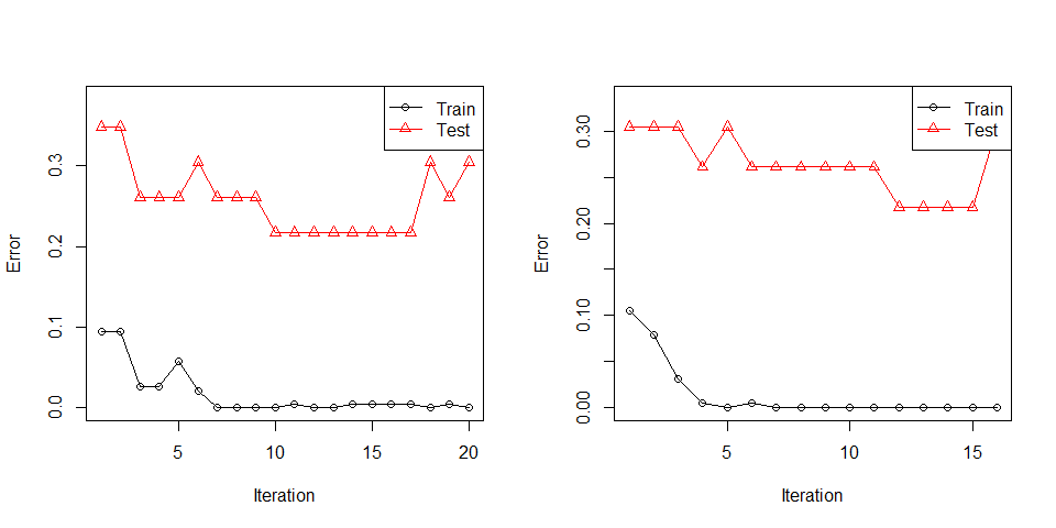
#> Warning in bb(x_train = x_train, y_train = y_train, classifier = classifier, :
#> Learning stopped at iteration 16
invisible(dev.off())
pred_discrete <- predict(object = m_discrete, newdata = x_test, type = "pred")
pred_real <- predict(object = m_real, newdata = x_test, type = "pred")

table(y_test, pred_discrete)
#>       pred_discrete
#> y_test 1 2 3 5 6 7
#>      1 6 1 0 0 0 0
#>      2 3 4 1 0 0 0
#>      3 1 0 1 0 0 0
#>      5 0 0 0 1 0 1
#>      6 0 0 0 0 1 0
#>      7 0 0 0 0 0 3
table(y_test, pred_real)
#>       pred_real
#> y_test 1 2 3 5 6 7
#>      1 7 0 0 0 0 0
#>      2 2 4 2 0 0 0
#>      3 2 0 0 0 0 0
#>      5 0 0 0 1 0 1
#>      6 0 0 0 0 1 0
#>      7 0 0 0 0 0 3
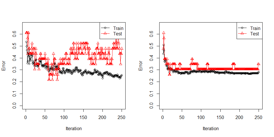
There is a major reason people use decision trees in boosting. It fits very quick. Let us try a pre-ready classifier Discrete Naive Bayes, “dnb”, in rbooster.
par(mfrow = c(1,2))
m_discrete <- booster(x_train = x_train,
                      y_train = y_train,
                      classifier = "dnb",
                      method = "discrete",
                      x_test = x_test,
                      y_test = y_test,
                      weighted_bootstrap = FALSE,
                      max_iter = 250,
                      lambda = 1,
                      print_detail = FALSE,
                      print_plot = TRUE,
                      bag_frac = 0.5,
                      p_weak = 4)

m_real <- booster(x_train = x_train,
                  y_train = y_train,
                  classifier = "dnb",
                  method = "real",
                  x_test = x_test,
                  y_test = y_test,
                  weighted_bootstrap = FALSE,
                  max_iter = 250,
                  lambda = 1e-4,
                  print_detail = FALSE,
                  print_plot = TRUE,
                  bag_frac = 0.2,
                  p_weak = 4)
invisible(dev.off())
pred_discrete <- predict(object = m_discrete, newdata = x_test, type = "pred")
pred_real <- predict(object = m_real, newdata = x_test, type = "pred")

table(y_test, pred_discrete)
#>       pred_discrete
#> y_test 1 2 3 5 6 7
#>      1 2 2 3 0 0 0
#>      2 2 5 0 0 0 1
#>      3 1 1 0 0 0 0
#>      5 0 0 0 1 0 1
#>      6 0 0 0 0 1 0
#>      7 0 0 0 0 0 3
table(y_test, pred_real)
#>       pred_real
#> y_test 1 2 3 5 6 7
#>      1 6 1 0 0 0 0
#>      2 4 4 0 0 0 0
#>      3 2 0 0 0 0 0
#>      5 0 0 0 1 0 1
#>      6 0 0 0 0 1 0
#>      7 0 0 0 0 0 3
I needed to play with lambda, bag_frac and p_weak a lot to find a good setting so that “dnb” fits. It is still not quite successful. Methods other that decision trees require care.
Custom Classifier
Classifier function requires x_train, y_train, weights as mandatory. Output of Classifier function will be the input for Predictor function. Predictor function requires model, which is the output of Classifier, x_new, which is the train features, and type inputs. type can only be “pred” or “prob”. “pred” must give a class vector of predictions, and “prob” must give a matrix of class probabilities. “pred” is mandatory for both Real and Discrete AdaBoost. However, Discrete AdaBoost does not require type “prob”. Let me prepare a made up Classifier function.
classifier_lm <- function(x_train, y_train, weights, ...){
  y_train_code <- c(-1,1)
  y_train_coded <- sapply(levels(y_train), function(m) y_train_code[(y_train == m) + 1])
  y_train_coded <- y_train_coded[,1]
  if (is.null(weights)) {
    weights <- rep(1, length(y_train))
  }

  model <- lm.wfit(x = as.matrix(cbind(1,x_train)), y = y_train_coded, w = weights)
  return(list(coefficients = model$coefficients,
              levels = levels(y_train)))
}

predictor_lm <- function(model, x_new, type = "pred", ...) {
  coef <- model$coefficients
  levels <- model$levels

  fit <- as.matrix(cbind(1, x_new))%*%coef
  probs <- 1/(1 + exp(-fit))
  probs <- data.frame(probs, 1 - probs)
  colnames(probs) <- levels

  if (type == "pred") {
    preds <- factor(levels[apply(probs, 1, which.max)], levels = levels, labels = levels)
    return(preds)
  }
  if (type == "prob") {
    return(probs)
  }
}
This classifier will convert y_train into (-1,1) codes and predictions will be transformed into the range (0,1) using logit transformation. These values will be used as probabilities and class with the higher probabilitiy will be selected as prediction. Since this is a linear classification method, it should work well with boosting. Let us see.
data <- glass0
p <- ncol(data) - 1

x <- data[,1:p]
y <- data[, p + 1]

train_i <- cv_sampler(y, 0.9)
x_train <- x[train_i,]
y_train <- y[train_i]

x_test <- x[-train_i,]
y_test <- y[-train_i]

par(mfrow = c(1,2))
m_discrete <- booster(x_train = x_train,
                      y_train = y_train,
                      classifier = classifier_lm,
                      predictor = predictor_lm,
                      method = "discrete",
                      x_test = x_test,
                      y_test = y_test,
                      weighted_bootstrap = FALSE,
                      max_iter = 600,
                      lambda = 2,
                      print_detail = FALSE,
                      print_plot = TRUE,
                      bag_frac = 0.4,
                      p_weak = 4)

m_real <- booster(x_train = x_train,
                  y_train = y_train,
                  classifier = classifier_lm,
                  predictor = predictor_lm,
                  method = "real",
                  x_test = x_test,
                  y_test = y_test,
                  weighted_bootstrap = FALSE,
                  max_iter = 200,
                  lambda = 0.1,
                  print_detail = FALSE,
                  print_plot = TRUE,
                  bag_frac = 1,
                  p_weak = 4)
#> Warning in bb(x_train = x_train, y_train = y_train, classifier = classifier, :
#> Learning stopped at iteration 45
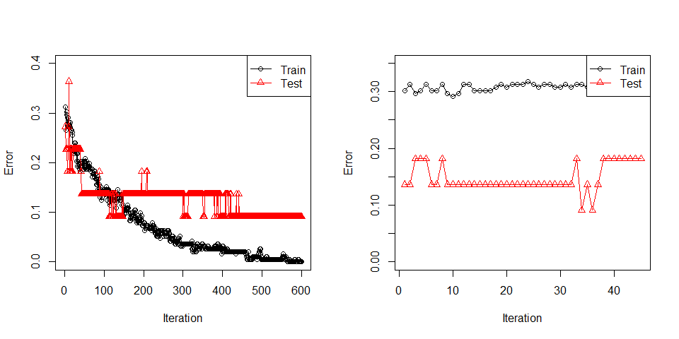
invisible(dev.off())
pred_discrete <- predict(object = m_discrete, newdata = x_test, type = "pred")
pred_real <- predict(object = m_real, newdata = x_test, type = "pred")

table(y_test, pred_discrete)
#>           pred_discrete
#> y_test     negative positive
#>   negative       14        1
#>   positive        1        6
table(y_test, pred_real)
#>           pred_real
#> y_test     negative positive
#>   negative       13        2
#>   positive        2        5
It fits but not quite there. print_plot can be set to FALSE. In that case, the same plot can be generated using plot function.
par(mfrow = c(1,2))
plot(m_discrete)
plot(m_real)

invisible(dev.off())
Pre-ready weak classifiers are “rpart”, “gnb”, “dnb”, “earth” and “glm” which are CART, Gaussian Naive Bayes, Discrete Naive Bayes, Multivariate Adaptive Regression Splines from earth package and logistic regression respectively. “glm” is not capable of multiclass classification. booster object can be used with prediction, plot, and print functions. For other details about booster object and its outputs, please see help document.