Tidy Presentation of Clinical Reporting.

reportRmd

The goal of reportRmd is to automate the reporting of clinical data in Rmarkdown environments. Functions include table one-style summary statistics, compilation of multiple univariate models, tidy output of multivariable models and side by side comparisons of univariate and multivariable models. Plotting functions include customisable survival curves, forest plots, and automated bivariate plots.

Installation

Installing from CRAN:

install.packages('reportRmd')

You can install the development version of reportRmd from GitHub with:

# install.packages("devtools")
devtools::install_github("biostatsPMH/reportRmd", ref="development")

New Features

• new compact summary table function rm_compactsum
• main functions are now pipeable
• new function to use variable labels in ggplots replace_plot_labels

Documentation

Online Documentation

Examples

Summary statistics by Sex

library(reportRmd)
data("pembrolizumab")

rm_covsum(data=pembrolizumab, maincov = 'sex',
covs=c('age','pdl1','change_ctdna_group'),
show.tests=TRUE)

Compact Table

pembrolizumab |> rm_compactsum( grp = 'sex',
xvars=c('age','pdl1','change_ctdna_group'))

Using Variable Labels

var_names <- data.frame(var=c("age","pdl1","change_ctdna_group"),
                          label=c('Age at study entry',
                                  'PD L1 percent',
                                  'ctDNA change from baseline to cycle 3'))

pembrolizumab <- set_labels(pembrolizumab,var_names)

rm_covsum(data=pembrolizumab, maincov = 'sex',
covs=c('age','pdl1','change_ctdna_group'))

Multiple Univariate Regression Analyses

rm_uvsum(data=pembrolizumab, response='orr',
covs=c('age','pdl1','change_ctdna_group'))
#> Waiting for profiling to be done...
#> Waiting for profiling to be done...
#> Waiting for profiling to be done...

Tidy multivariable analysis

glm_fit <- glm(orr~change_ctdna_group+pdl1+cohort,
               family='binomial',
               data = pembrolizumab)
rm_mvsum(glm_fit,showN=T)

Combining univariate and multivariable models

uvsumTable <- rm_uvsum(data=pembrolizumab, response='orr',
covs=c('age','sex','pdl1','change_ctdna_group'),tableOnly = TRUE)
#> Waiting for profiling to be done...
#> Waiting for profiling to be done...
#> Waiting for profiling to be done...
#> Waiting for profiling to be done...

glm_fit <- glm(orr~change_ctdna_group+pdl1,
               family='binomial',
               data = pembrolizumab)
mvsumTable <- rm_mvsum(glm_fit,tableOnly = TRUE)

rm_uv_mv(uvsumTable,mvsumTable)

Simple survival summary table

Shows events, median survival, survival rates at different times and the log rank test. Does not allow for covariates or strata, just simple tests between groups

 rm_survsum(data=pembrolizumab,time='os_time',status='os_status',
 group="cohort",survtimes=c(12,24),
# group="cohort",survtimes=seq(12,36,12),
# survtimesLbls=seq(1,3,1),
 survtimesLbls=c(1,2),
 survtimeunit='yr')

Summarise Cumulative incidence

library(survival)
data(pbc)
rm_cifsum(data=pbc,time='time',status='status',group=c('trt','sex'),
eventtimes=c(1825,3650),eventtimeunit='day')
#> 106 observations with missing data were removed.

Plotting survival curves

ggkmcif2(response = c('os_time','os_status'),
cov='cohort',
data=pembrolizumab)

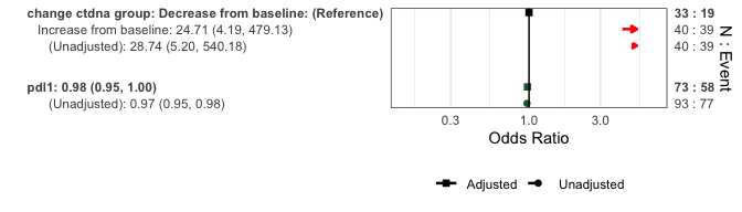
Plotting odds ratios

require(ggplot2)
#> Loading required package: ggplot2
forestplotMV(glm_fit)
#> Warning in forestplotMV(glm_fit): NAs introduced by coercion

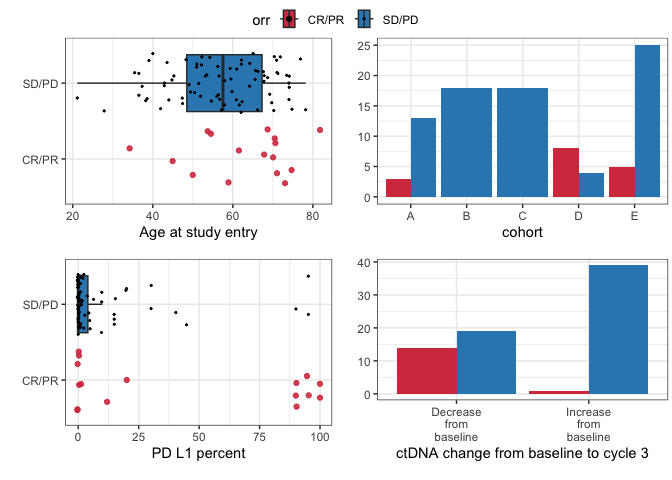
Plotting bivariate relationships

These plots are designed for quick inspection of many variables, not for publication.

require(ggplot2)
plotuv(data=pembrolizumab, response='orr',
covs=c('age','cohort','pdl1','change_ctdna_group'))
#> Boxplots not shown for categories with fewer than 20 observations.
#> Boxplots not shown for categories with fewer than 20 observations.

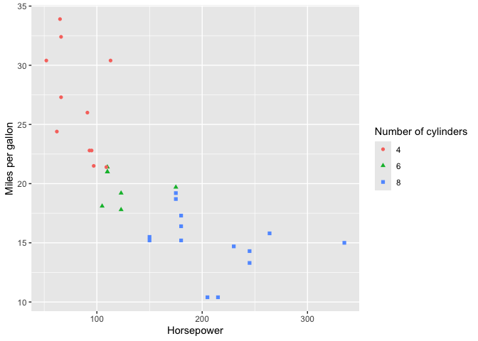
Replacing variable names with labels in ggplot

data("mtcars")
mtcars <- mtcars |> 
  dplyr::mutate(cyl = as.factor(cyl)) |>
  set_labels(data.frame(var=c("hp","mpg","cyl"),
                        label=c('Horsepower',
                                'Miles per gallon',
                                'Number of cylinders'))) 
p <- mtcars |> 
ggplot(aes(x=hp, y=mpg, color=cyl, shape=cyl)) +
    geom_point()
replace_plot_labels(p)