Convert Images to Usable Color Schemes.
:rainbow: schemr package
Convert photos into useable colour schemes
schemr is an R package for turning your photos into usable colour schemes for R visualisations.
The key driver is the image_to_pallette function, which:
- reads in images;
- finds colour blobs within the image, representing the key highlighting colours; and
- uses affinity propagation clustering to condense the set of key colours.
:hammer: Installing schemr
Install the latest CRAN version of schemr by:
install.packages("schemr")
Alternatively, install the development version of schemr can be installed by running:
devtools::install_github("stuart-morrison/schemr")
:camera: Photo example
First we have a look at a photo of my beautiful old car.
library(OpenImageR)
library(magrittr)

# Read in the image
image <- readImage(path = "images/car.jpg")

# Shrink down the image - Note resizeImage width and height are on array dimensions, rather than on image dimensions
new_height <- dim(image)[1] * 0.5
new_width <- dim(image)[2] * 0.5
image %<>% resizeImage(image = ., width = new_height, height = new_width)

# Plot
plot(as.raster(image))

We see big blobs of blue, yellow and orange. Using schemr to extract these, we get:
library(schemr)

# Extract key colours from image
# I use the median to extract the centre of each 'blob' - but any function summary function, eg, mean, max, min, will all work
schemr_data <- image_to_pallette(image_path = "images/car.jpg", resize_factor = 0.5,
                                  verbose = FALSE, summary_method = median)

# Plot the image
plot(schemr_data)

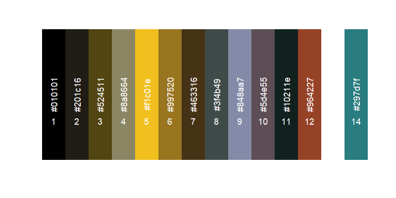
We can see the palette of colours found in the image by using the palette method on the schemr data.
palette(schemr_data)

In addition, printing the class, shows the vector of hex RGB codes that make up the clustered data:
schemr_data
## [1] "#010101" "#201c16" "#524511" "#8a8664" "#f1c01e"
## [6] "#997520" "#463316" "#3f4b49" "#848aa7" "#5d4e55"
## [11] "#10211e" "#964227" "#ffffff" "#297d7f"
:bar_chart: Using schemr palettes in plots
The evaluated palette is easy to apply immediately into data visualisation by access through the palette attribute.
library(ggplot2)
# Example plot using the iris data set
ggplot() +
    geom_point(data = iris,
               aes(x = Petal.Length, y = Petal.Width,
                   col = Species),
               size = 4) +
    scale_color_manual(name = "Species",
                       values = schemr_data$palette[c(5, 12, 14)]) +
    labs(x = "Petal length", y = "Petal width") +
    theme_bw(base_size = 18)

:raised_hands: Colour space conversions
schemr also contains functions to convert colour data both to and from the following colour spaces:
| From\To | RGB | XYZ | Lab | HSL | HSV |
|---|---|---|---|---|---|
| RGB | :white_check_mark: | :white_check_mark: | :white_check_mark: | :white_check_mark: | |
| XYZ | :white_check_mark: | :white_check_mark: | :white_check_mark: | :white_check_mark: | |
| Lab | :white_check_mark: | :white_check_mark: | :white_check_mark: | :white_check_mark: | |
| HSL | :white_check_mark: | :white_check_mark: | :white_check_mark: | :white_check_mark: | |
| HSV | :white_check_mark: | :white_check_mark: | :white_check_mark: | :white_check_mark: |
Colour conversion constants and functions are provided for sRGB and Adobe 1998 RGB spaces, with user ability to apply other conversions for other RGB spaces.
For example, using excellent colours from the wesanderson package:
library(wesanderson)

# Extract some lovely Zissou colours
colour_hex <- wes_palettes$Zissou1

# Convert to Lab space
colour_lab <- hex_to_lab(hex = colour_hex, transformation = "Adobe")

# Convert Lab space to XYZ space
colour_xyz <- lab_to_xyz(lab = colour_lab)

# Convert XYZ space to RGB colour channels
colour_rgb <- xyz_to_rgb(xyz = colour_xyz, transformation = "Adobe")