Balancing Multiclass Datasets for Classification Tasks.

scutr: SMOTE and Cluster-Based Undersampling Technique in R

Imbalanced training datasets impede many popular classifiers. To balance training data, a combination of oversampling minority classes and undersampling majority classes is necessary. This package implements the SCUT (SMOTE and Cluster-based Undersampling Technique) algorithm, which uses model-based clustering and synthetic oversampling to balance multiclass training datasets.

This implementation only works on numeric training data and works best when there are more than two classes. For binary classification problems, other packages may be better suited.

The original SCUT paper uses SMOTE (essentially linear interpolation between points) for oversampling and expectation maximization clustering, which fits a mixture of Gaussian distributions to the data. These are the default methods in scutr, but random oversampling as well as some distance-based undersampling techniques are available.

Installation

You can install the released version of scutr from CRAN with:

install.packages("scutr")

And the development version from GitHub with:

# install.packages("devtools")
devtools::install_github("s-kganz/scutr")

Example Usage

We start with an imbalanced dataset that comes with the package.

library(scutr)
data(imbalance)
imbalance <- imbalance[imbalance$class %in% c(2, 3, 19, 20), ]
imbalance$class <- as.numeric(imbalance$class)

plot(imbalance$V1, imbalance$V2, col=imbalance$class)

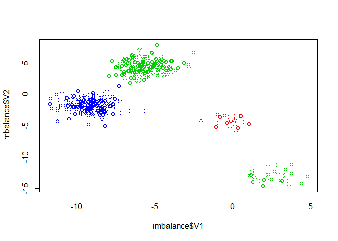
table(imbalance$class)
#> 
#>   2   3  19  20 
#>  20  30 190 200

Then, we apply SCUT with SMOTE oversampling and k-means clustering with seven clusters.

scutted <- SCUT(imbalance, "class", undersample = undersample_kmeans,
                usamp_opts = list(k=7))
plot(scutted$V1, scutted$V2, col=scutted$class)

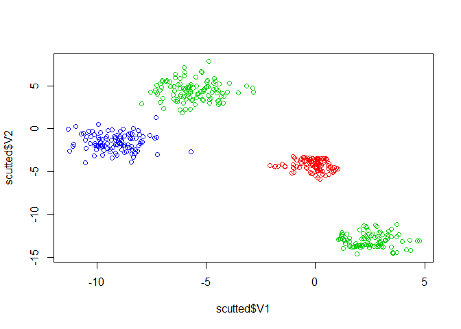
table(scutted$class)
#> 
#>   2   3  19  20 
#> 110 110 110 110

The dataset is now balanced and we have retained the distribution of the data.