Superpixel Segmentation with the Simple Non-Iterative Clustering Algorithm.

snic

Efficient superpixel segmentation for multi-band imagery using the Simple Non-Iterative Clustering (SNIC) algorithm. The package wraps a C++ implementation with an ergonomic R interface, integrates with terra for raster workflows, and provides helpers for seed placement, plotting, and reproducibility.

Installation

The snic package can be installed from CRAN:

install.packages("snic")

Or the development version from GitHub:

# install.packages("remotes")
remotes::install_github("rolfsimoes/snic")

The terra package is suggested for raster support and required for most of the plotting utilities demonstrated below.

Highlights

• Implements SNIC with a fast C++ core exposed to R
• Works with in-memory arrays or terra::SpatRaster objects
• Offers multiple seeding strategies via snic_grid(type = c("rectangular", "diamond", "hexagonal", "random")) and interactive placement via snic_grid_manual()
• Includes ready-to-plot utilities (snic_plot()) for quick inspection of inputs, seeds, and resulting segments

Requirements

• Raster support.terra (>= 1.7) is suggested and is required for every raster example below. In-memory array workflows can skip it, but you will lose the quick plotting helpers.
• Animation support.magick is optional and only needed for snic_animation(). The chunk is cached so missing the package merely skips the demo.

Why SNIC?

SNIC produces compact superpixels in near-linear time and avoids the iterative updates of SLIC-like algorithms. The snic package exposes those speed benefits through:

• A C++ core that processes moderate Sentinel-2 tiles (thousands x thousands of pixels x multiple bands) in a few seconds on a laptop.
• Native terra integration, so you keep CRS, extent, and metadata intact.
• Reproducible seeding helpers, which makes parameter sweeps easy to script and compare.

Pipeline overview

The SNIC workflow is short and reproducible:

• Step 1 - Seed placement. Select or draw a grid of starting seeds that guide where the superpixels will grow. Grids can be generated automatically with snic_grid() (rectangular, diamond, hexagonal, or random layouts) or crafted interactively with snic_grid_manual().
• Step 2 - Segmentation. Run snic() with the chosen seeds to grow superpixels and inspect the result with snic_plot() or the animated helper snic_animation().

Quick start

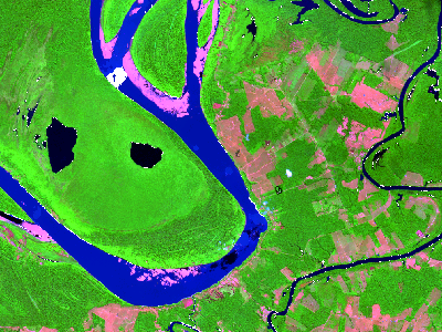
The example below demonstrates a typical SNIC workflow with the bundled Sentinel-2 subset.

library(snic)
library(terra)

# Sentinel-2 subset packaged with snic
data_dir <- system.file("demo-geotiff", package = "snic", mustWork = TRUE)
bands <- c("B02", "B04", "B08", "B12")
paths <- file.path(
  data_dir,
  sprintf("S2_20LMR_%s_20220630.tif", bands)
)
s2 <- terra::rast(paths)
names(s2) <- bands

# Visualise RGB composite with superpixel boundaries
snic_plot(
  s2,
  r = "B12", g = "B08", b = "B02",
  stretch = "lin"
)

Step 1 - Seed placement

Seed placement controls the number, shape, and location of the resulting superpixels. The package ships with several grid generators, each returning a two-column (r, c) matrix ready for snic():

• snic_grid(type = "rectangular") - equally spaced seeds along rows and columns.
• snic_grid(type = "diamond") - staggered rows produce a diagonal pattern that better respects gradients.
• snic_grid(type = "hexagonal") - hexagonal tiling for more isotropic superpixels.
• snic_grid(type = "random") - jittered seeds when structure is irregular or prior knowledge is limited.

Use snic_count_seeds() to forecast how many superpixels a spacing will produce before running the algorithm.

set.seed(42)

grid_types <- c("rectangular", "diamond", "hexagonal", "random")
seed_examples <- lapply(grid_types, function(tp) {
    snic_grid(s2, type = tp, spacing = 30L, padding = 0L)
  }
)

op <- par(mfrow = c(2, 2), mar = c(1.5, 1.5, 2, 1))

for (i in seq_along(seed_examples)) {
  snic_plot(
    s2,
    r = 4, g = 3, b = 1,
    stretch = "lin",
    seeds = seed_examples[[i]],
    seeds_plot_args = list(pch = 3, col = "#F6D55C", lwd = 2)
  )
  title(grid_types[i])
}

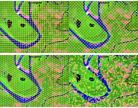
snic_count_seeds(s2, spacing = 30L)
#> [1] 850

par(op)

Interactive placement

Automatic grids get you started quickly, but experts can refine seeds interactively. snic_grid_manual() opens a plotting device where you can add, move, or remove seeds on-the-fly and then feed the result straight into snic():

manual_seeds <- snic_grid_manual(
  s2,
  base_seeds = seeds_rect,
  r = 4, g = 3, b = 1,
  stretch = "lin"
)

seg_manual <- snic(
  s2,
  seeds = manual_seeds,
  compactness = 0.1
)

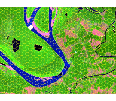
Step 2 - SNIC segmentation

Once seeds are defined, pass them to snic() together with the imagery and a compactness factor. The result is a labeled raster that can be visualized alongside the seeds for validation.

seg_hex <- snic(s2, seeds = seed_examples[[3L]], compactness = 0.2)

snic_plot(
  s2,
  r = "B12", g = "B08", b = "B02",
  stretch = "lin",
  seg = seg_hex,
  seg_plot_args = list(border = "#FFFF00", col = NA, lwd = 0.6)
)

Animated seeding review

snic_animation() replays the seeding process, adding one seed per frame, re-running snic(), and composing the frames into a GIF. Cache the chunk so the animation is generated only once.

if (!requireNamespace("magick", quietly = TRUE)) {
  stop("Install the 'magick' package to render the animation.")
}

unlink("man/figures/segmentation-animation.gif")

set.seed(123)
animation_seeds <- snic_grid(s2, type = "random", spacing = 20L, padding = 0L)

gif_path <- snic_animation(
  s2,
  seeds = animation_seeds,
  file_path = "man/figures/segmentation-animation.gif",
  max_frames = 20L,
  delay = 30,
  r = 4, g = 3, b = 1,
  stretch = "lin",
  seeds_plot_args = list(pch = 16, col = "#00FFFF", cex = 1),
  seg_plot_args = list(border = "#FFD700", col = NA, lwd = 0.6),
  snic_args = list(compactness = 0.1),
  device_args = list(height = 192, width = 256, res = 120, bg = "white")
)

Contributing

Bug reports, feature requests, and pull requests are welcome in the issue tracker. When proposing changes:

• Run R CMD check or devtools::check() to keep the package stable.
• Re-knit README.Rmd if you touch code chunks so plots stay in sync.
• Mention whether raster dependencies (terra, magick) were available when reproducing a bug, as it affects plotting and animation paths.