Optimal Histogram Binning Using Shimazaki-Shinomoto Method.

sshist

The sshist package implements the Shimazaki-Shinomoto method for finding the optimal number of bins in histograms.

Unlike the standard Freedman-Diaconis rule (used by default in ggplot2), this method minimizes the expected L2 loss function between the histogram and the unknown underlying density function. It is particularly effective for:

• Time-dependent rate estimation (PSTH).
• Identifying intrinsic data structures in multimodal distributions.
• Optimizing both 1D and 2D data binnings.

Installation

# stable version from CRAN
install.packages("sshist")

You can install the development version of sshist like so:

# install.packages("devtools")
devtools::install_github("celebithil/sshist")

Example 1: Basic 1D Usage

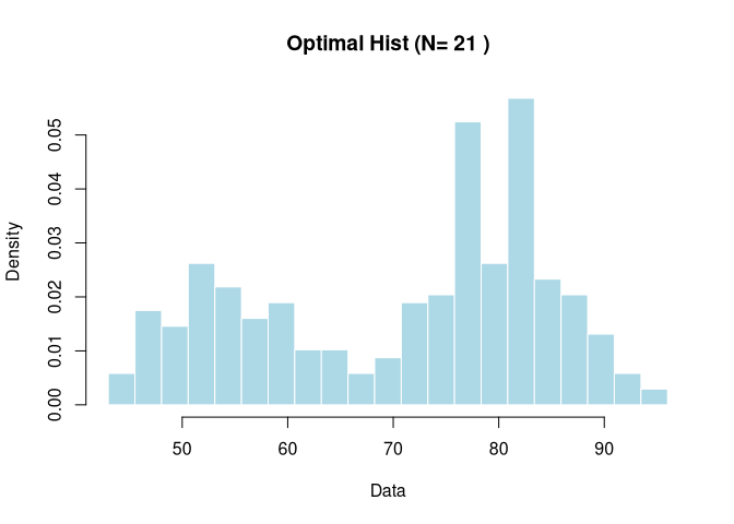
Here is a basic example using the Old Faithful Geyser data.

library(sshist)

# Load data
data(faithful)
x_data <- faithful$waiting

# Calculate optimal binning
res <- sshist(x_data)

# Print summary
print(res)
#> Shimazaki-Shinomoto Histogram Optimization
#> ------------------------------------------
#> Optimal Bins (N): 21 
#> Bin Width (D):    2.524 
#> Cost Minimum:     -8.525

hist(res$data, breaks=res$edges, freq=FALSE,
       main=paste("Optimal Hist (N=", res$opt_n, ")"),
       col="lightblue", border="white", xlab="Data")

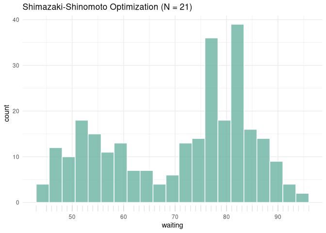
Example 2: Integration with ggplot2

sshist calculates the optimal parameters, which you can easily pass to ggplot2.

library(ggplot2)

# Create a data frame
df <- data.frame(waiting = x_data)

ggplot(df, aes(x = waiting)) +
  geom_histogram(breaks = res$edges, fill = "#69b3a2", color = "white", alpha = 0.8) +
  geom_rug(alpha = 0.1) +
  ggtitle(paste0("Shimazaki-Shinomoto Optimization (N = ", res$opt_n, ")")) +
  theme_minimal()

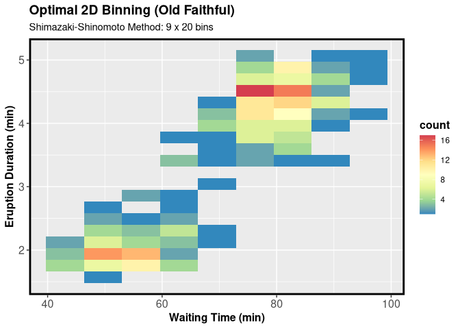
Example 3: 2D Histogram Optimization

For bivariate data, sshist_2d finds the optimal binning for both X and Y axes simultaneously.

# Get bimodal 2D data
y_data <- faithful$eruptions

# Optimize
res2d <- sshist_2d(x_data, y_data)

# Print summary
print(res2d)
#> Shimazaki-Shinomoto 2D Histogram Optimization
#> ---------------------------------------------
#> Optimal Bins X:   9 
#> Optimal Bins Y:   20 
#> Bin Width X:      5.889 
#> Bin Width Y:      0.175 
#> Cost Minimum:     -5.717

Example 4: 2D Optimization with ggplot2

You can easily use the optimized bin counts from sshist_2d in ggplot2 by passing them to the bins argument in geom_bin2d.

# We use the 'res2d' object calculated in Example 3
# containing optimal bins for Old Faithful data

res2d <- sshist_2d(faithful$waiting, faithful$eruptions )

ggplot(faithful, aes(waiting, eruptions)) +
  geom_bin2d(bins = c(res2d$opt_nx, res2d$opt_ny)) +
  scale_fill_distiller(palette = "Spectral") +
  labs(
    title = "Optimal 2D Binning (Old Faithful)",
    subtitle = paste0("Shimazaki-Shinomoto Method: ", 
                      res2d$opt_nx, " x ", res2d$opt_ny, " bins"),
    x = "Waiting Time (min)",
    y = "Eruption Duration (min)"
  ) +
  theme(axis.text = element_text(size = 12),
        title = element_text(size = 12,face="bold"),
        panel.border = element_rect(linewidth = 2, color = "black", fill = NA))

References

• Shimazaki, H. and Shinomoto, S., 2007. A method for selecting the bin size of a time histogram. Neural Computation, 19(6), pp.1503-1527. doi:10.1162/neco.2007.19.6.1503
• https://www.neuralengine.org/res/histogram.html
• https://github.com/shimazaki/density_estimation
• https://s-shinomoto.com/toolbox/sshist/hist.html.