Description

Estimate Step Counts from 'Accelerometry' Data.

Description

Interfaces the 'stepcount' Python module <https://github.com/OxWearables/stepcount> to estimate step counts and other activities from 'accelerometry' data.

README.md

cran.r-project.org

stepcount

The goal of stepcount is to wrap up the https://github.com/OxWearables/stepcount algorithm.

Installation

Install `stepcount` Python Module

See https://github.com/OxWearables/stepcount?tab=readme-ov-file#install for how to install the stepcount python module.

In R, you can do this via:

envname = "stepcountblah"
reticulate::conda_create(envname = envname, packages = c("python=3.9", "openjdk", "pip"))
Sys.unsetenv("RETICULATE_PYTHON")
reticulate::use_condaenv(envname)
reticulate::py_install("stepcount", envname = envname, method = "conda", pip = TRUE)

Once this is finished, you should be able to check this via:

stepcount::have_stepcount_condaenv()
stepcount::have_stepcount()

In some cases, you ay want to set RETICULATE_PYTHON variable:

stepcount::unset_reticulate_python()
clist = reticulate::conda_list()
Sys.setenv(RETICULATE_PYTHON = clist$python[clist$name == "stepcount"])
stepcount::use_stepcount_condaenv()

Issues

If you are using the Random Forest model from stepcount, you may need hmmlearn<0.3.0 due to some issues with its new implementation of its models as described https://github.com/OxWearables/stepcount/issues/62 (Feb 2024).

Install `stepcount` R Package

You can install the development version of stepcount from GitHub with:

# install.packages("devtools")
devtools::install_github("jhuwit/stepcount")

Usage

Loading the `stepcount` conda environment

In order to use the stepcount conda environment that OxWearables recommends, you must run this command before reticulate is loaded:

stepcount::use_stepcount_condaenv()

The `RETICULATE_PYTHON` environment variable

If you have the RETICULATE_PYTHON environment variable in your .Renviron or your PATH, then reticulate will still use that version of Python and the code will likely not work. The unset_reticulate_python() function will unset that environment variable. So the usage would start with something like:

stepcount::unset_reticulate_python()
stepcount::use_stepcount_condaenv()

and if you need reticulate, you would load it after

stepcount::unset_reticulate_python()
stepcount::use_stepcount_condaenv()
library(reticulate)

The stepcount_check function can determine if the stepcount module can be loaded

stepcount::stepcount_check()
#> [1] TRUE

Running `stepcount` (file)

The main function is stepcount::stepcount, which takes can take in a file directly:

library(stepcount)
library(dplyr)
#> 
#> Attaching package: 'dplyr'
#> The following objects are masked from 'package:stats':
#> 
#>     filter, lag
#> The following objects are masked from 'package:base':
#> 
#>     intersect, setdiff, setequal, union
library(ggplot2)
library(tidyr)
#> Warning: package 'tidyr' was built under R version 4.3.2
file = system.file("extdata/P30_wrist100.csv.gz", package = "stepcount")
if (stepcount_check()) {
  out = stepcount(file = file)
}
#> Loading model...
#> Downloading https://wearables-files.ndph.ox.ac.uk/files/models/stepcount/ssl-20230208.joblib.lzma...
#> Gravity calibration...Gravity calibration... Done! (0.05s)
#> Nonwear detection...Nonwear detection... Done! (0.04s)
#> Resampling...Resampling... Done! (0.05s)
#> Predicting from Model
#> Running step counter...
#> Defining windows...
#> Using local /Users/johnmuschelli/miniconda3/envs/stepcount/lib/python3.9/site-packages/stepcount/torch_hub_cache/OxWearables_ssl-wearables_v1.0.0
#> Classifying windows...
#> Processing Result

Let’s see inside the output, which is a list of values, namely a data.frame of steps with the time (in 10s increments) and the number of steps in those 10 seconds, a data.frame named walking which has indicators for if there is walking within that 10 second period:

names(out)
#> [1] "steps"            "walking"          "step_times"       "summary"         
#> [5] "summary_adjusted" "info"
str(out)
#> List of 6
#>  $ steps           :'data.frame':    361 obs. of  2 variables:
#>   ..$ time : POSIXct[1:361], format: "2019-07-22 14:34:45" "2019-07-22 14:34:55" ...
#>   ..$ steps: num [1:361] 0 0 0 0 0 0 0 0 0 0 ...
#>  $ walking         :'data.frame':    361 obs. of  2 variables:
#>   ..$ time   : POSIXct[1:361], format: "2019-07-22 14:34:45.88" "2019-07-22 14:34:55.88" ...
#>   ..$ walking: num [1:361] 0 0 0 0 0 0 0 0 0 0 ...
#>  $ step_times      :'data.frame':    5739 obs. of  1 variable:
#>   ..$ time: chr [1:5739] "2019-07-22 14:36:26.4899" "2019-07-22 14:36:26.9566" "2019-07-22 14:36:27.4899" "2019-07-22 14:36:27.9566" ...
#>  $ summary         :List of 16
#>   ..$ total         : int 5739
#>   ..$ hourly        : int [1:2(1d)] 2424 3315
#>   .. ..- attr(*, "dimnames")=List of 1
#>   .. .. ..$ : chr [1:2] "2019-07-22 14:00:00" "2019-07-22 15:00:00"
#>   ..$ daily_stats   :'data.frame':   1 obs. of  5 variables:
#>   .. ..$ Walk(mins): num 54
#>   .. ..$ Steps     : num 5739
#>   .. ..$ StepsQ1At : chr "14:49:45"
#>   .. ..$ StepsQ2At : chr "15:06:45"
#>   .. ..$ StepsQ3At : chr "15:20:55"
#>   .. ..- attr(*, "pandas.index")=DatetimeIndex(['2019-07-22'], dtype='datetime64[ns]', name='time', freq='D')
#>   ..$ daily_avg     : int 5739
#>   ..$ daily_med     : int 5739
#>   ..$ daily_min     : int 5739
#>   ..$ daily_max     : int 5739
#>   ..$ total_walk    : int 54
#>   ..$ daily_walk_avg: int 54
#>   ..$ daily_walk_med: int 54
#>   ..$ daily_walk_min: int 54
#>   ..$ daily_walk_max: int 54
#>   ..$ cadence_peak1 : int 123
#>   ..$ cadence_peak30: int 113
#>   ..$ daily_QAt_avg : chr [1:3(1d)] "14:49:45" "15:06:45" "15:20:55"
#>   .. ..- attr(*, "dimnames")=List of 1
#>   .. .. ..$ : chr [1:3] "StepsQ1At" "StepsQ2At" "StepsQ3At"
#>   ..$ daily_QAt_med : chr [1:3(1d)] "14:49:45" "15:06:45" "15:20:55"
#>   .. ..- attr(*, "dimnames")=List of 1
#>   .. .. ..$ : chr [1:3] "StepsQ1At" "StepsQ2At" "StepsQ3At"
#>  $ summary_adjusted:List of 16
#>   ..$ total         : num NaN
#>   ..$ hourly        : num [1:24(1d)] NaN NaN NaN NaN NaN NaN NaN NaN NaN NaN ...
#>   .. ..- attr(*, "dimnames")=List of 1
#>   .. .. ..$ : chr [1:24] "2019-07-22 00:00:00" "2019-07-22 01:00:00" "2019-07-22 02:00:00" "2019-07-22 03:00:00" ...
#>   ..$ daily_stats   :'data.frame':   1 obs. of  5 variables:
#>   .. ..$ Walk(mins): num NaN
#>   .. ..$ Steps     : num NaN
#>   .. ..$ StepsQ1At : num NaN
#>   .. ..$ StepsQ2At : num NaN
#>   .. ..$ StepsQ3At : num NaN
#>   .. ..- attr(*, "pandas.index")=DatetimeIndex(['2019-07-22'], dtype='datetime64[ns]', name='time', freq='D')
#>   ..$ daily_avg     : num NaN
#>   ..$ daily_med     : num NaN
#>   ..$ daily_min     : num NaN
#>   ..$ daily_max     : num NaN
#>   ..$ total_walk    : num NaN
#>   ..$ daily_walk_avg: num NaN
#>   ..$ daily_walk_med: num NaN
#>   ..$ daily_walk_min: num NaN
#>   ..$ daily_walk_max: num NaN
#>   ..$ cadence_peak1 : int 124
#>   ..$ cadence_peak30: int 114
#>   ..$ daily_QAt_avg : num [1:3(1d)] NaN NaN NaN
#>   .. ..- attr(*, "dimnames")=List of 1
#>   .. .. ..$ : chr [1:3] "StepsQ1At" "StepsQ2At" "StepsQ3At"
#>   ..$ daily_QAt_med : num [1:3(1d)] NaN NaN NaN
#>   .. ..- attr(*, "dimnames")=List of 1
#>   .. .. ..$ : chr [1:3] "StepsQ1At" "StepsQ2At" "StepsQ3At"
#>  $ info            :List of 12
#>   ..$ Filename             : chr "/Library/Frameworks/R.framework/Versions/4.3-x86_64/Resources/library/stepcount/extdata/P30_wrist100.csv.gz"
#>   ..$ Device               : chr ".csv"
#>   ..$ Filesize(MB)         : num 4.8
#>   ..$ SampleRate           : int 100
#>   ..$ CalibOK              : int 0
#>   ..$ CalibErrorBefore(mg) : num NaN
#>   ..$ CalibErrorAfter(mg)  : num NaN
#>   ..$ WearTime(days)       : num 0.0417
#>   ..$ NonwearTime(days)    : num 0
#>   ..$ NumNonwearEpisodes   : int 0
#>   ..$ ResampleRate         : int 30
#>   ..$ NumTicksAfterResample: int 108001
head(out$steps)
#>                  time steps
#> 1 2019-07-22 14:34:45     0
#> 2 2019-07-22 14:34:55     0
#> 3 2019-07-22 14:35:05     0
#> 4 2019-07-22 14:35:15     0
#> 5 2019-07-22 14:35:25     0
#> 6 2019-07-22 14:35:35     0
tail(out$steps)
#>                    time steps
#> 356 2019-07-22 15:33:55    20
#> 357 2019-07-22 15:34:05    20
#> 358 2019-07-22 15:34:15    20
#> 359 2019-07-22 15:34:25    19
#> 360 2019-07-22 15:34:35    17
#> 361 2019-07-22 15:34:45   NaN
tail(out$walking)
#>                    time walking
#> 356 2019-07-22 15:33:55       1
#> 357 2019-07-22 15:34:05       1
#> 358 2019-07-22 15:34:15       1
#> 359 2019-07-22 15:34:25       1
#> 360 2019-07-22 15:34:35       1
#> 361 2019-07-22 15:34:45     NaN

The step_timesdata.frame indicates which times are when steps occurred (at the original sample rate). Make sure you have the digits.secs option set to see the sub-seconds for the times (esp for writing out files in readr::write_csv):

head(out$step_times)
#>                       time
#> 1 2019-07-22 14:36:26.4899
#> 2 2019-07-22 14:36:26.9566
#> 3 2019-07-22 14:36:27.4899
#> 4 2019-07-22 14:36:27.9566
#> 5 2019-07-22 14:36:30.4566
#> 6 2019-07-22 14:36:30.8233
options(digits.secs = 3)
head(out$step_times)
#>                       time
#> 1 2019-07-22 14:36:26.4899
#> 2 2019-07-22 14:36:26.9566
#> 3 2019-07-22 14:36:27.4899
#> 4 2019-07-22 14:36:27.9566
#> 5 2019-07-22 14:36:30.4566
#> 6 2019-07-22 14:36:30.8233

We can plot a portion of the tri-axial data and show where the steps were indicated:

df = readr::read_csv(file)
#> Rows: 360001 Columns: 5
#> ── Column specification ────────────────────────────────────────────────────────
#> Delimiter: ","
#> dbl  (4): x, y, z, annotation
#> dttm (1): time
#> 
#> ℹ Use `spec()` to retrieve the full column specification for this data.
#> ℹ Specify the column types or set `show_col_types = FALSE` to quiet this message.
if (stepcount_check()) {
  st = out$step_times
    dat = df[10000:12000,] %>%
      dplyr::select(-annotation) %>%
      tidyr::gather(axis, value, -time)
    st = st %>%
      dplyr::mutate(time = lubridate::as_datetime(time)) %>%
      dplyr::as_tibble()
    st = st %>%
      dplyr::filter(time >= min(dat$time) & time <= max(dat$time))
    dat %>%
      ggplot2::ggplot(ggplot2::aes(x = time, y = value, colour = axis)) +
      ggplot2::geom_line() +
      ggplot2::geom_vline(data = st, ggplot2::aes(xintercept = time))
}

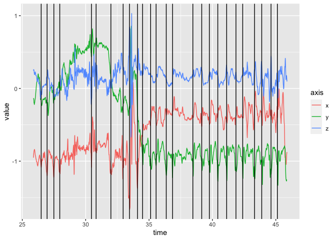
The main caveat is that stepcount is very precise in the format of the data, primarily it must have the columns time, x, y, and z in the data.

Running `stepcount` (data frame)

Alternatively, you can pass out a data.frame, rename the columns to what you need them to be and then run stepcount on that:

head(df)
#> # A tibble: 6 × 5
#>   time                         x      y      z annotation
#>   <dttm>                   <dbl>  <dbl>  <dbl>      <dbl>
#> 1 2019-07-22 14:34:45.890 -0.735 -0.274 -0.481          0
#> 2 2019-07-22 14:34:45.900 -0.591 -0.330 -0.466          0
#> 3 2019-07-22 14:34:45.910 -0.468 -0.496 -0.529          0
#> 4 2019-07-22 14:34:45.920 -0.389 -0.750 -0.670          0
#> 5 2019-07-22 14:34:45.930 -0.369 -1.00  -0.949          0
#> 6 2019-07-22 14:34:45.940 -0.371 -1.17  -1.36           0
out_df = stepcount(file = df)
#> Writing file to CSV...
#> Loading model...
#> Gravity calibration...Gravity calibration... Done! (0.04s)
#> Nonwear detection...Nonwear detection... Done! (0.03s)
#> Resampling...Resampling... Done! (0.06s)
#> Predicting from Model
#> Running step counter...
#> Defining windows...
#> Using local /Users/johnmuschelli/miniconda3/envs/stepcount/lib/python3.9/site-packages/stepcount/torch_hub_cache/OxWearables_ssl-wearables_v1.0.0
#> Classifying windows...
#> Processing Result

Which gives same output for this data:

all.equal(out[c("steps", "walking", "step_times")],
          out_df[c("steps", "walking", "step_times")])
#> [1] TRUE

Running `stepcount` on multiple files

When you pass in multiple files, stepcount will run all of them, but it will only load the model once, which can have savings, but the results are still in memory:

if (stepcount_check()) {
  out2 = stepcount(file = c(file, file))
  length(out2)
  names(out2)
  # all.equal(out[c("steps", "walking", "step_times")], 
  #           out2[[1]][c("steps", "walking", "step_times")])
}
#> Loading model...
#> Gravity calibration...Gravity calibration... Done! (0.04s)
#> Nonwear detection...Nonwear detection... Done! (0.04s)
#> Resampling...Resampling... Done! (0.06s)
#> Predicting from Model
#> Running step counter...
#> Defining windows...
#> Using local /Users/johnmuschelli/miniconda3/envs/stepcount/lib/python3.9/site-packages/stepcount/torch_hub_cache/OxWearables_ssl-wearables_v1.0.0
#> Classifying windows...
#> Processing Result
#> Gravity calibration...Gravity calibration... Done! (0.04s)
#> Nonwear detection...Nonwear detection... Done! (0.04s)
#> Resampling...Resampling... Done! (0.06s)
#> Predicting from Model
#> Running step counter...
#> Defining windows...
#> Using local /Users/johnmuschelli/miniconda3/envs/stepcount/lib/python3.9/site-packages/stepcount/torch_hub_cache/OxWearables_ssl-wearables_v1.0.0
#> Classifying windows...
#> Processing Result
#> NULL

Stepcount Random Forest

The model_type parameter indicates the type of model being run, and the rf will provide the predictions from a random forest

if (stepcount_check()) {
  out_rf = stepcount(file = file, model_type = "rf")
}

r-stepcount

stepcount

Installation

Install `stepcount` Python Module

Issues

Install `stepcount` R Package

Usage

Loading the `stepcount` conda environment

The `RETICULATE_PYTHON` environment variable

Running `stepcount` (file)

Running `stepcount` (data frame)

Running `stepcount` on multiple files

Stepcount Random Forest

Version

License

Status

Source

Homepage

Platforms (77)

stepcount

Installation

Install stepcount Python Module

Issues

Install stepcount R Package

Usage

Loading the stepcount conda environment

The RETICULATE_PYTHON environment variable

Running stepcount (file)

Running stepcount (data frame)

Running stepcount on multiple files

Stepcount Random Forest

Version

License

Status

Source

Homepage

Platforms77 (77)

Install `stepcount` Python Module

Install `stepcount` R Package

Loading the `stepcount` conda environment

The `RETICULATE_PYTHON` environment variable

Running `stepcount` (file)

Running `stepcount` (data frame)

Running `stepcount` on multiple files

Platforms (77)