Quickly Explore Complex Survey Data.
Surveyexplorer
Visualize and tabulate single-choice, multiple-choice, matrix-style questions from survey data. Includes ability to group cross-tabulations, frequency distributions, and plots by categorical variables and to integrate survey weights. Ideal for quickly uncovering descriptive patterns in survey data.
Installation
install.packages("surveyexplorer")
# or devtools::install_github("liamhaller/surveyexplorer") for the devlopment version
Examples
library(surveyexplorer)
The data used in the following examples is from the berlinbears dataset, a fictional survey of bears in Berlin, that is included in the surveyexplorer package.
Single-choice questions
#Basic table
single_table(berlinbears,
             question = income)
| Question: income | ||
| n | freq | |
|---|---|---|
| <1000 | 82 | 0.164 |
| 1000-2000 | 50 | 0.100 |
| 2000-3000 | 177 | 0.354 |
| 3000-4000 | 109 | 0.218 |
| 5000+ | 57 | 0.114 |
| No answer | 22 | 0.044 |
| NA | 3 | 0.006 |
| Column Total | 500 | — |
Use group_by = to partition the question into several groups
single_table(berlinbears,
             question = income,
             group_by = gender)
| Question: income | ||||||||
| grouped by: gender | ||||||||
| female | male | NA | Rowwise Total | |||||
|---|---|---|---|---|---|---|---|---|
| Frequency | Count | Frequency | Count | Frequency | Count | Frequency | Count | |
| <1000 | 16.74% | 39 | 15.73% | 39 | 21.05% | 4 | 16.40% | 82 |
| 1000-2000 | 9.87% | 23 | 9.68% | 24 | 15.79% | 3 | 10.00% | 50 |
| 2000-3000 | 35.62% | 83 | 35.89% | 89 | 26.32% | 5 | 35.40% | 177 |
| 3000-4000 | 21.89% | 51 | 22.18% | 55 | 15.79% | 3 | 21.80% | 109 |
| 5000+ | 11.59% | 27 | 10.89% | 27 | 15.79% | 3 | 11.40% | 57 |
| No answer | 3.86% | 9 | 4.84% | 12 | 5.26% | 1 | 4.40% | 22 |
| NA | 0.43% | 1 | 0.81% | 2 | 0.00% | 0 | 0.60% | 3 |
| Columnwise Total | 46.60% | 233 | 49.60% | 248 | 3.80% | 19 | 100.00% | 500 |
Ignore unwanted subgroups with subgroups_to_exclude
single_table(berlinbears,
             question = income,
             group_by = gender,
             subgroups_to_exclude = NA)
| Question: income | ||||||
| grouped by: gender | ||||||
| female | male | Rowwise Total | ||||
|---|---|---|---|---|---|---|
| Frequency | Count | Frequency | Count | Frequency | Count | |
| <1000 | 16.74% | 39 | 15.73% | 39 | 16.22% | 78 |
| 1000-2000 | 9.87% | 23 | 9.68% | 24 | 9.77% | 47 |
| 2000-3000 | 35.62% | 83 | 35.89% | 89 | 35.76% | 172 |
| 3000-4000 | 21.89% | 51 | 22.18% | 55 | 22.04% | 106 |
| 5000+ | 11.59% | 27 | 10.89% | 27 | 11.23% | 54 |
| No answer | 3.86% | 9 | 4.84% | 12 | 4.37% | 21 |
| NA | 0.43% | 1 | 0.81% | 2 | 0.62% | 3 |
| Columnwise Total | 48.44% | 233 | 51.56% | 248 | 100.00% | 481 |
Remove NAs from the question variable with na.rm
single_table(berlinbears,
             question = income,
             group_by = gender,
             subgroups_to_exclude = NA,
             na.rm = TRUE)
| Question: income | ||||||
| grouped by: gender | ||||||
| female | male | Rowwise Total | ||||
|---|---|---|---|---|---|---|
| Frequency | Count | Frequency | Count | Frequency | Count | |
| <1000 | 16.81% | 39 | 15.85% | 39 | 16.32% | 78 |
| 1000-2000 | 9.91% | 23 | 9.76% | 24 | 9.83% | 47 |
| 2000-3000 | 35.78% | 83 | 36.18% | 89 | 35.98% | 172 |
| 3000-4000 | 21.98% | 51 | 22.36% | 55 | 22.18% | 106 |
| 5000+ | 11.64% | 27 | 10.98% | 27 | 11.30% | 54 |
| No answer | 3.88% | 9 | 4.88% | 12 | 4.39% | 21 |
| Columnwise Total | 48.54% | 232 | 51.46% | 246 | 100.00% | 478 |
Finally, you can specify survey weights using the weight option
single_table(berlinbears,
             question = income,
             group_by = gender,
             subgroups_to_exclude = NA,
             na.rm = TRUE,
             weights = weights)
| Question: income | ||||||
| grouped by: gender | ||||||
| female | male | Rowwise Total | ||||
|---|---|---|---|---|---|---|
| Frequency | Count | Frequency | Count | Frequency | Count | |
| <1000 | 15.96% | 59.6 | 17.21% | 75.2 | 16.63% | 134.8 |
| 1000-2000 | 10.46% | 39.1 | 10.19% | 44.5 | 10.31% | 83.6 |
| 2000-3000 | 33.79% | 126.3 | 33.88% | 148.0 | 33.84% | 274.3 |
| 3000-4000 | 25.08% | 93.7 | 25.34% | 110.7 | 25.22% | 204.4 |
| 5000+ | 9.82% | 36.7 | 8.68% | 37.9 | 9.21% | 74.6 |
| No answer | 4.90% | 18.3 | 4.70% | 20.5 | 4.79% | 38.8 |
| Columnwise Total | 46.10% | 373.6 | 53.90% | 436.9 | 100.00% | 810.5 |
| Frequencies and counts are weighted | ||||||
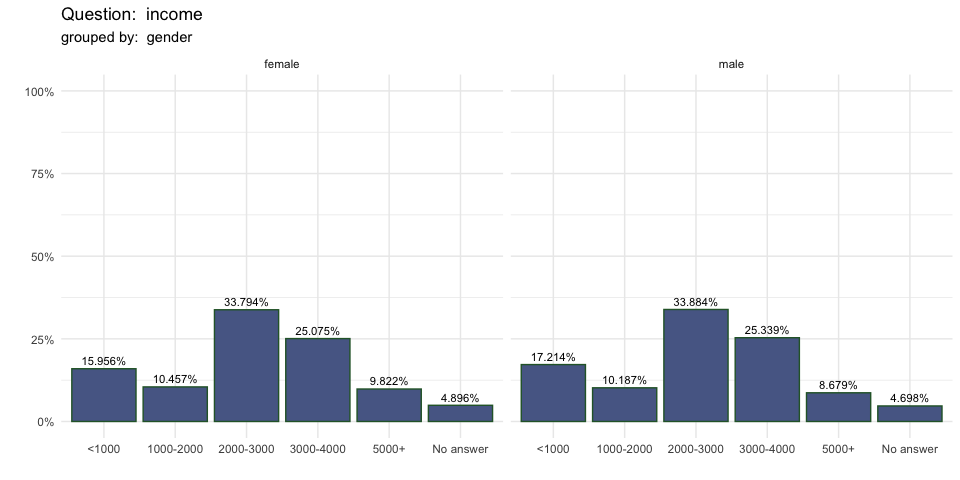
The same syntax can be applied to the single_freq function to plot frequencies of the question optionally partitioned by subgroups.
single_freq(berlinbears,
             question = income,
             group_by = gender,
             subgroups_to_exclude = NA,
             na.rm = TRUE,
             weights = weights)
Multiple-choice questions
The options and syntax for multiple-choice tables multi_table and graphs multi_graphs are the same. The only difference is the question input also accommodates tidyselect syntax to select several columns for each answer option. For example, the question “will_eat” has five answer options each prefixed by “will_eat”
berlinbears |>
  dplyr::select(starts_with('will_eat')) |>
  head()
#>   will_eat.SQ001 will_eat.SQ002 will_eat.SQ003 will_eat.SQ004 will_eat.SQ005
#> 1              0              1              0              1              1
#> 2              0              1              1              1              1
#> 3              1              1              0              1              1
#> 4              0              0              0              1              0
#> 5              0              0              0              1              1
#> 6              0              0              0              1              0
The same syntax can be used to select the question for the multiple choice tables and graphs
multi_table(berlinbears,
            question = dplyr::starts_with('will_eat'),
            group_by = genus,
            subgroups_to_exclude = NA,
            na.rm = TRUE)
| Question: dplyr::starts_with("will_eat") | ||||||
| grouped by: genus | ||||||
| Ailuropoda | Ursus | Rowwise Total | ||||
|---|---|---|---|---|---|---|
| Frequency | Count | Frequency | Count | Frequency | Count | |
| will_eat.SQ004 | 97.54% | 278 | 91.62% | 175 | 40.12% | 453 |
| will_eat.SQ002 | 59.30% | 169 | 66.49% | 127 | 26.22% | 296 |
| will_eat.SQ005 | 43.86% | 125 | 46.60% | 89 | 18.95% | 214 |
| will_eat.SQ001 | 24.91% | 71 | 27.23% | 52 | 10.89% | 123 |
| will_eat.SQ003 | 8.42% | 24 | 9.95% | 19 | 3.81% | 43 |
| Columnwise Total | 59.08% | 667 | 40.92% | 462 | 100.00% | 1129 |
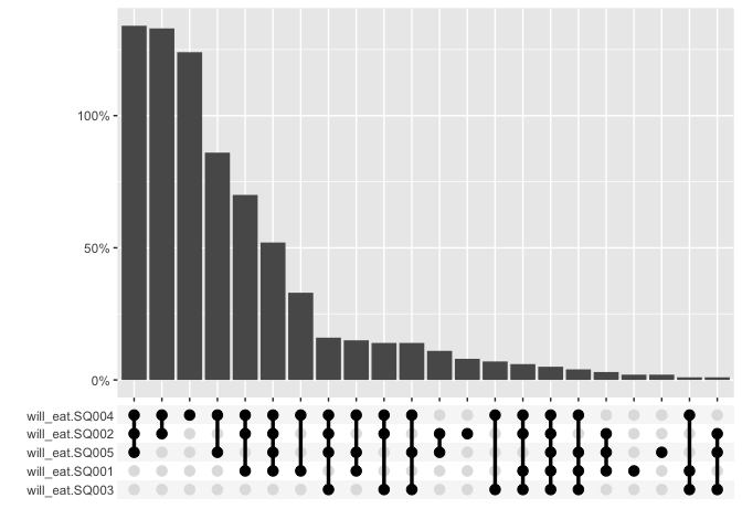
For graphing, the multi_freq function creates an UpSet plot to visualize the frequencies of the intersecting sets for each answer combination and also includes the ability to specify weights.
multi_freq(berlinbears,
            question = dplyr::starts_with('will_eat'),
            na.rm = TRUE,
            weights = weights)
#> Estimes are only preciese to one significant digit, weights may have been rounded
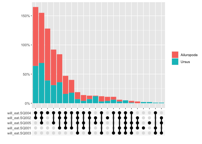
The graphs can also be grouped
multi_freq(berlinbears,
            question = dplyr::starts_with('will_eat'),
            group_by = genus,
            subgroups_to_exclude = NA,
            na.rm = FALSE,
            weights = weights)
#> Estimes are only preciese to one significant digit, weights may have been rounded
Matrix Questions
matrix_table has the same syntax as above and works with array or categorical questions
matrix_table(berlinbears,
             dplyr::starts_with('c_'),
             group_by = is_parent)
| Question: dplyr::starts_with("c_") | ||||
| grouped by: is_parent | ||||
| high | low | medium | NA | |
|---|---|---|---|---|
| 0 | ||||
| c_diet | 6.02% (20) | 71.99% (239) | 16.57% (55) | 5.42% (18) |
| c_exercise | 25% (83) | 27.71% (92) | 24.1% (80) | 23.19% (77) |
| 1 | ||||
| c_diet | 3.57% (6) | 75% (126) | 17.26% (29) | 4.17% (7) |
| c_exercise | 19.05% (32) | 27.38% (46) | 23.81% (40) | 29.76% (50) |
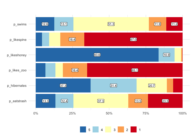
matrix_freq visualizes the frequencies of responses
matrix_freq(berlinbears,
             dplyr::starts_with('p_'),
             na.rm = TRUE)
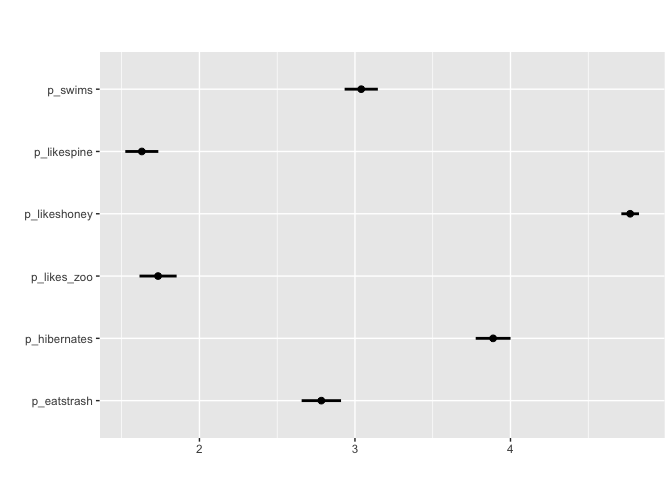
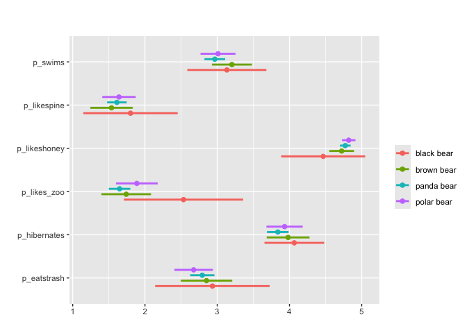
For array/matrix style questions that are numeric matrix_mean plots the mean values and confidence intervals
matrix_mean(berlinbears,
             question = dplyr::starts_with('p_'),
             na.rm = TRUE)
#Can also apply grouping + survey weights
matrix_mean(berlinbears,
            question = dplyr::starts_with('p_'),
            na.rm = TRUE,
            group_by = species,
            subgroups_to_exclude = NA)
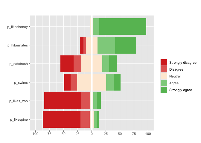
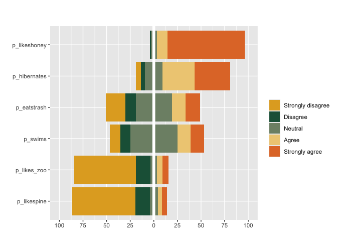
Finally, for Likert questions (scales of 3,5,7,9…) matrix_likert provides a custom plot
#you can specify custom labels with the `label` argument
matrix_likert(berlinbears,
              question = dplyr::starts_with('p_'),
              labels = c('Strongly disagree', 'Disagree','Neutral','Agree','Strongly agree'))
#can also apply pass custom colors and specify weights weights
matrix_likert(berlinbears,
              question = dplyr::starts_with('p_'),
              labels = c('Strongly disagree', 'Disagree','Neutral','Agree','Strongly agree'),
              colors = c("#E1AA28", "#1E5F46", "#7E8F75", "#EFCD83", "#E17832"),
              weights = weights)
Overview
Functions
- Single-choice
single_tablesingle_freq
- Multiple-choice
multi_tablemulti_freq
- Matrix
matrix_tablematrix_freqmatrix_meanmatrix_likert
*_table functions return a gt table of the cross tabulations and frequencies for each question while *_freq returns the same data but as a plot.
For matrix-style questions with numerical input, matrix_mean plots the mean value value and ± two standard deviations. matrix_likert visualizes questions that accept Likert responses (strongly agree-strongly disagree) or questions with 3,5,7,9… categories.
Syntax
Each function contains the following options
- dataset —The input dataframe (or tibble) of survey questions
- question — The column(s) that contain the response options for a question, can be selected by using tidyselect semantics or providing a vector of column names or numbers
- group_by — Optional variable to group the analysis. If provided, the frequencies and counts will be calculated within each subgroup
- subgroups_to_exclude — Optional vector specifying subgroups to exclude from the analysis
- weights — Optional variable containing survey weights. If provided, frequencies and counts will be weighted accordingly
- na.rm — Logical indicating whether to remove NA values from question before analysis.