Estimation of the ROC Curve and the AUC for Complex Survey Data.
svyROC
The goal of the svyROC package is to plot weighted estimates of the ROC curves and to obtain weighted estimates of the AUC.
The following functions are available:
wse,wsp: estimate sensitivity and specificity parameters for a specific cut-off point considering sampling weights.wroc: estimate the ROC curve considering sampling weights.wauc: estimate the AUC considering sampling weights.corrected.wauc: correct the optimism of the weighted estimate of the AUC by means of replicate weights.wocp: calculate optimal cut-off points for individual classification considering sampling weights.wroc.plot: plot the ROC curve.
The methodology proposed for the above-mentioned functions can be found in the following references:
Iparragirre, A., Barrio, I., Aramendi, J. and Arostegui, I. (2022). Estimation of cut-off points under complex-sampling design data. SORT-Statistics and Operations Research Transactions46(1), 137–158.
Iparragirre, A., Barrio, I. and Arostegui, I. (2023). Estimation of the ROC curve and the area under it with complex survey data. Stat12(1), e635.
Iparragirre, A. and Barrio, I. (2024). Optimism Correction of the AUC with Complex Survey Data. In: Einbeck, J., Maeng, H., Ogundimu, E., Perrakis, K. (eds) Developments in Statistical Modelling. IWSM 2024. Contributions to Statistics. Springer, Cham.
Installation
To install the package from CRAN:
install.packages("svyROC")
To install the most updated version of the package from GitHub run the following code:
devtools::install_github("aiparragirre/svyROC")
Example
We need information on three elements for each unit in the sample in order to estimate the ROC curve (wroc() function) and AUC (wauc() function):
response.var: variable indicating the dichotomous response variable.phat.var: predicted probabilities of event.weights.var: variable indicating the sampling weights.
We can put these three vectors in a data frame, or save them separately in three different vectors. The data set example_data_wroc is set as an example in the package. We also need to define the tags for events and non-events.
library(svyROC)
data(example_data_wroc)

mycurve <- wroc(response.var = "y", phat.var = "phat", weights.var = "weights",
                data = example_data_wroc,
                tag.event = 1, tag.nonevent = 0)

# Or equivalently
mycurve <- wroc(response.var = example_data_wroc$y,
                phat.var = example_data_wroc$phat,
                weights.var = example_data_wroc$weights,
                tag.event = 1, tag.nonevent = 0)
Similarly, we can run the following code to estimate the AUC:
auc.obj <- wauc(response.var = "y",
                phat.var = "phat",
                weights.var = "weights",
                tag.event = 1,
                tag.nonevent = 0,
                data = example_data_wroc)

# Or equivalently
auc.obj <- wauc(response.var = example_data_wroc$y,
                phat.var = example_data_wroc$phat,
                weights.var = example_data_wroc$weights,
                tag.event = 1, tag.nonevent = 0)
We can correct the optimism of the weighted estimate of the AUC by means of replicate weights, as proposed in Iparragirre and Barrio (2024), by means of the corrected.wauc() function. For this purpose, we additionally need information on the covariates and the sampling design. Here is an example of the usage of this function:
data(example_variables_wroc)
mydesign <- survey::svydesign(ids = ~cluster, strata = ~strata,
                              weights = ~weights, nest = TRUE,
                              data = example_variables_wroc)
m <- survey::svyglm(y ~ x1 + x2 + x3 + x4 + x5 + x6, design = mydesign,
                    family = quasibinomial())
phat <- predict(m, newdata = example_variables_wroc, type = "response")
myaucw <- wauc(response.var = example_variables_wroc$y, phat.var = phat,
               weights.var = example_variables_wroc$weights)

# Correction of the AUCw:
set.seed(1)
cor <- corrected.wauc(data = example_variables_wroc,
                      formula = y ~ x1 + x2 + x3 + x4 + x5 + x6,
                      tag.event = 1, tag.nonevent = 0,
                      weights.var = "weights", strata.var = "strata", cluster.var = "cluster",
                      method = "dCV", dCV.method = "pooling", k = 10, R = 20)
# Or equivalently:
set.seed(1)
cor <- corrected.wauc(design = mydesign,
                      formula = y ~ x1 + x2 + x3 + x4 + x5 + x6,
                      tag.event = 1, tag.nonevent = 0,
                      method = "dCV", dCV.method = "pooling", k = 10, R = 20)
We can also estimate the sensitivity (wse()) and specificity (wsp()) parameters for a specific cut-off point considering sampling weights. For this purpose, we need to indicate the cut-off point we want to use in the function by means of the argument cutoff.value:
# Specificity ----------------------------------------------------------

sp.obj <- wsp(response.var = "y",
              phat.var = "phat",
              weights.var = "weights",
              tag.nonevent = 0,
              cutoff.value = 0.5,
              data = example_data_wroc)

# Or equivalently
sp.obj <- wsp(response.var = example_data_wroc$y,
              phat.var = example_data_wroc$phat,
              weights.var = example_data_wroc$weights,
              tag.nonevent = 0,
              cutoff.value = 0.5)

# Sensitivity ----------------------------------------------------------

se.obj <- wse(response.var = "y",
              phat.var = "phat",
              weights.var = "weights",
              tag.event = 1,
              cutoff.value = 0.5,
              data = example_data_wroc)

# Or equivalently
se.obj <- wse(response.var = example_data_wroc$y,
              phat.var = example_data_wroc$phat,
              weights.var = example_data_wroc$weights,
              tag.event = 1,
              cutoff.value = 0.5)
Finally, use the function wocp() to obtain optimal cut-off points for individual classification as proposed in Iparragirre et al (2022). Some functions of the package OptimalCutpoints have been modified in order for them to consider sampling weights:
Lopez-Raton, M., Rodriguez-Alvarez, M.X, Cadarso-Suarez, C. and Gude-Sampedro, F. (2014). OptimalCutpoints: An R Package for Selecting Optimal Cutpoints in Diagnostic Tests. Journal of Statistical Software61(8), 1–36.
One of the methods proposed in the paper needs to be selected when running the function by means of the argument method: Youden, MaxProdSpSe, ROC01 or MaxEfficiency.
myocp <- wocp(response.var = "y",
              phat.var = "phat", weights.var = "weights",
              tag.event = 1,
              tag.nonevent = 0,
              method = "Youden",
              data = example_data_wroc)

# Or equivalently
myocp <- wocp(example_data_wroc$y,
              example_data_wroc$phat,
              example_data_wroc$weights,
              tag.event = 1,
              tag.nonevent = 0,
              method = "Youden")
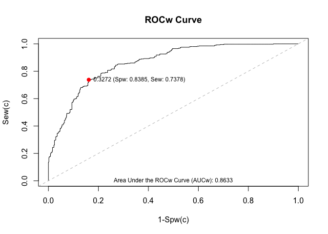
If you want to draw the optimal cut-off point in the ROC curve, then use the function wroc.plot() and indicate the method by means of the argument cutoff.method in the function wroc() as follows:
mycurve <- wroc(response.var = "y",
                phat.var = "phat",
                weights.var = "weights",
                data = example_data_wroc,
                tag.event = 1,
                tag.nonevent = 0,
                cutoff.method = "Youden")
wroc.plot(x = mycurve,
          print.auc = TRUE,
          print.cutoff = TRUE)