Speedy Word Embedding Association Test and Extras Using R.
sweater 
The goal of sweater (Speedy Word Embedding Association Test & Extras using R) is to test for associations among words in word embedding spaces. The methods provided by this package can also be used to test for unwanted associations, or biases.
The package provides functions that are speedy. They are either implemented in C++, or are speedy but accurate approximation of the original implementation proposed by Caliskan et al (2017). See the benchmark here.
This package provides extra methods such as Relative Norm Distance, Embedding Coherence Test, SemAxis and Relative Negative Sentiment Bias.
If your goal is to reproduce the analysis in Caliskan et al (2017), please consider using the original Java program or the R package cbn by Lowe. To reproduce the analysis in Garg et al (2018), please consider using the original Python program. To reproduce the analysis in Mazini et al (2019), please consider using the original Python program.
Please cite this software as:
Chan, C., (2022). sweater: Speedy Word Embedding Association Test and Extras Using R. Journal of Open Source Software, 7(72), 4036, https://doi.org/10.21105/joss.04036
For a BibTeX entry, use the output from citation(package = "sweater").
Installation
Recommended: install the latest development version
remotes::install_github("gesistsa/sweater")
or the “stable” release
install.packages("sweater")
Notation of a query
All tests in this package use the concept of queries (see Badilla et al., 2020) to study associations in the input word embeddings w. This package uses the “STAB” notation from Brunet et al (2019). [1]
All tests depend on two types of words. The first type, namely, S_words and T_words, is target words (or neutral words in Garg et al). In the case of studying biases, these are words that should have no bias. For instance, the words such as “nurse” and “professor” can be used as target words to study the gender bias in word embeddings. One can also separate these words into two sets, S_words and T_words, to group words by their perceived bias. For example, Caliskan et al. (2017) grouped target words into two groups: mathematics (“math”, “algebra”, “geometry”, “calculus”, “equations”, “computation”, “numbers”, “addition”) and arts (“poetry”, “art”, “dance”, “literature”, “novel”, “symphony”, “drama”, “sculpture”). Please note that also T_words is not always required.
The second type, namely A_words and B_words, is attribute words (or group words in Garg et al). These are words with known properties in relation to the bias that one is studying. For example, Caliskan et al. (2017) used gender-related words such as “male”, “man”, “boy”, “brother”, “he”, “him”, “his”, “son” to study gender bias. These words qualify as attribute words because we know they are related to a certain gender.
It is recommended using the function query() to make a query and calculate_es() to calculate the effect size.
Available methods
| Target words | Attribute words | Method | method argument | Suggested by query? | legacy functions [2] |
|---|---|---|---|---|---|
| S_words | A_words | Mean Average Cosine Similarity (Mazini et al. 2019) | “mac” | yes | mac(), mac_es() |
| S_words | A_words, B_words | Relative Norm Distance (Garg et al. 2018) | “rnd” | yes | rnd(), rnd_es() |
| S_words | A_words, B_words | Relative Negative Sentiment Bias (Sweeney & Najafian. 2019) | “rnsb” | no | rnsb(), rnsb_es() |
| S_words | A_words, B_words | Embedding Coherence Test (Dev & Phillips. 2019) | “ect” | no | ect(), ect_es(), plot_ect() |
| S_words | A_words, B_words | SemAxis (An et al. 2018) | “semaxis” | no | semaxis() |
| S_words | A_words, B_words | Normalized Association Score (Caliskan et al. 2017) | “nas” | no | nas() |
| S_words, T_words | A_words, B_words | Word Embedding Association Test (Caliskan et al. 2017) | “weat” | yes | weat(), weat_es(), weat_resampling(), weat_exact() |
| S_words, T_words | A_words, B_words | Word Embeddings Fairness Evaluation (Badilla et al. 2020) | To be implemented |
Example: Mean Average Cosine Similarity
The simplest form of bias detection is Mean Average Cosine Similarity (Mazini et al. 2019). The same method was used in Kroon et al. (2020). googlenews is a subset of the pretrained word2vec word embeddings provided by Google.
By default, the query() function guesses the method you want to use based on the combination of target words and attribute words provided (see the “Suggested?” column in the above table). You can also make this explicit by specifying the method argument. Printing the returned object shows the effect size (if available) as well as the functions that can further process the object: calculate_es and plot. Please read the help file of calculate_es (?calculate_es) on what is the meaning of the effect size for a specific test.
require(sweater)
S1 <- c("janitor", "statistician", "midwife", "bailiff", "auctioneer",
"photographer", "geologist", "shoemaker", "athlete", "cashier",
"dancer", "housekeeper", "accountant", "physicist", "gardener",
"dentist", "weaver", "blacksmith", "psychologist", "supervisor",
"mathematician", "surveyor", "tailor", "designer", "economist",
"mechanic", "laborer", "postmaster", "broker", "chemist", "librarian",
"attendant", "clerical", "musician", "porter", "scientist", "carpenter",
"sailor", "instructor", "sheriff", "pilot", "inspector", "mason",
"baker", "administrator", "architect", "collector", "operator",
"surgeon", "driver", "painter", "conductor", "nurse", "cook",
"engineer", "retired", "sales", "lawyer", "clergy", "physician",
"farmer", "clerk", "manager", "guard", "artist", "smith", "official",
"police", "doctor", "professor", "student", "judge", "teacher",
"author", "secretary", "soldier")

A1 <- c("he", "son", "his", "him", "father", "man", "boy", "himself",
"male", "brother", "sons", "fathers", "men", "boys", "males",
"brothers", "uncle", "uncles", "nephew", "nephews")

## The same as:
## mac_neg <- query(googlenews, S_words = S1, A_words = A1, method = "mac")
mac_neg <- query(googlenews, S_words = S1, A_words = A1)
mac_neg
#>
#> ── sweater object ──────────────────────────────────────────────────────────────
#> Test type:  mac
#> Effect size:  0.1375856
#>
#> ── Functions ───────────────────────────────────────────────────────────────────
#> • `calculate_es()`: Calculate effect size
#> • `plot()`: Plot the bias of each individual word
The returned object is an S3 object. Please refer to the help file of the method for the definition of all slots (in this case: ?mac). For example, the magnitude of bias for each word in S1 is available in the P slot.
sort(mac_neg$P)
#>         sales      designer     economist       manager      clerical
#>  -0.002892495   0.039197285   0.046155954   0.047322071   0.048912403
#>      operator administrator        author    auctioneer        tailor
#>   0.050275206   0.050319552   0.051470909   0.065440629   0.074771460
#>     secretary     librarian     scientist  statistician         pilot
#>   0.077506781   0.079040760   0.082535536   0.088000351   0.088337791
#>     geologist      official     architect        broker     professor
#>   0.088567238   0.090706054   0.091598653   0.098761198   0.101847166
#>      engineer     collector         smith       chemist      surveyor
#>   0.103448025   0.104596505   0.104956871   0.110798023   0.112098241
#>     inspector        weaver     physicist       midwife    supervisor
#>   0.112383017   0.113221694   0.114302092   0.115791724   0.118784135
#>     physician        artist     conductor        clergy         guard
#>   0.118990813   0.119571390   0.120602413   0.123313906   0.128804364
#>    accountant    instructor         judge    postmaster         nurse
#>   0.131700192   0.133135210   0.135238197   0.138497652   0.143781092
#>          cook     attendant       sheriff        dancer  photographer
#>   0.145019382   0.149134946   0.149992633   0.150637430   0.151388282
#>  psychologist       cashier       surgeon mathematician       retired
#>   0.151908676   0.153591372   0.158348402   0.158969004   0.165010593
#>         clerk       student        porter      gardener       dentist
#>   0.165903226   0.167006052   0.172551327   0.173346664   0.174776368
#>       teacher       athlete       bailiff       painter        driver
#>   0.175027901   0.176353551   0.176440157   0.176625091   0.181269327
#>         baker     shoemaker        lawyer    blacksmith        farmer
#>   0.183320490   0.183548112   0.189963886   0.198764788   0.199243319
#>         mason        police   housekeeper        sailor      musician
#>   0.203577329   0.206264491   0.208280255   0.208689761   0.219184802
#>       janitor      mechanic        doctor       soldier       laborer
#>   0.220953800   0.224008333   0.226657160   0.238053858   0.251032714
#>     carpenter
#>   0.259775292
Example: Relative Norm Distance
This analysis reproduces the analysis in Garg et al (2018), namely Figure 1.
B1 <- c("she", "daughter", "hers", "her", "mother", "woman", "girl",
"herself", "female", "sister", "daughters", "mothers", "women",
"girls", "females", "sisters", "aunt", "aunts", "niece", "nieces"
)

garg_f1 <- query(googlenews, S_words = S1, A_words = A1, B_words = B1)
garg_f1
#>
#> ── sweater object ──────────────────────────────────────────────────────────────
#> Test type:  rnd
#> Effect size:  -6.341598
#>
#> ── Functions ───────────────────────────────────────────────────────────────────
#> • `calculate_es()`: Calculate effect size
#> • `plot()`: Plot the bias of each individual word
The object can be plotted by the function plot to show the bias of each word in S. Words such as “nurse”, “midwife” and “librarian” are more associated with female, as indicated by the positive relative norm distance.
plot(garg_f1)
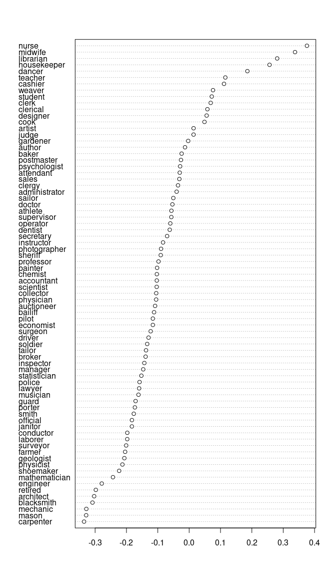
The effect size is simply the sum of all relative norm distance values (Equation 3 in Garg et al. 2018). It is displayed simply by printing the object. You can also use the function calculate_es to obtain the numeric result.
The more positive effect size indicates that words in S_words are more associated with B_words. As the effect size is negative, it indicates that the concept of occupation is more associated with A_words, i.e. male.
calculate_es(garg_f1)
#> [1] -6.341598
Example: SemAxis
This analysis attempts to reproduce the analysis in An et al. (2018).
You may obtain the word2vec word vectors trained with Trump supporters Reddit from here. This package provides a tiny version of the data small_reddit for reproducing the analysis.
S2 <- c("mexicans", "asians", "whites", "blacks", "latinos")
A2 <- c("respect")
B2 <- c("disrespect")
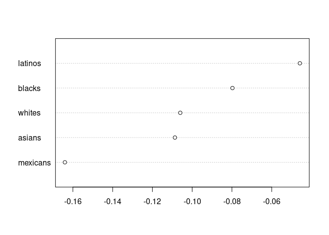
res <- query(small_reddit, S_words = S2, A_words = A2, B_words = B2, method = "semaxis", l = 1)
plot(res)
Example: Embedding Coherence Test
Embedding Coherence Test (Dev & Phillips, 2019) is similar to SemAxis. The only significant difference is that no “SemAxis” is calculated (the difference between the average word vectors of A_words and B_words). Instead, it calculates two separate axes for A_words and B_words. Then it calculates the proximity of each word in S_words with the two axes. It is like doing two separate mac, but ect averages the word vectors of A_words / B_words first.
It is important to note that P is a 2-D matrix. Hence, the plot is 2-dimensional. Words above the equality line are more associated with B_words and vice versa.
res <- query(googlenews, S_words = S1, A_words = A1, B_words = B1, method = "ect")
res$P
#>           janitor statistician   midwife   bailiff auctioneer photographer
#> A_words 0.3352883   0.13495237 0.1791162 0.2698131 0.10123085    0.2305419
#> B_words 0.2598501   0.08300127 0.3851766 0.2331852 0.06957685    0.2077952
#>          geologist shoemaker   athlete   cashier    dancer housekeeper
#> A_words 0.13817054 0.2842002 0.2607956 0.2340296 0.2282981   0.3205498
#> B_words 0.05101061 0.1850456 0.2570477 0.3171645 0.3508183   0.4610773
#>         accountant  physicist  gardener   dentist    weaver blacksmith
#> A_words  0.2029543 0.17446868 0.2657907 0.2672548 0.1767915  0.3080301
#> B_words  0.1789482 0.08362829 0.2873140 0.2623802 0.2475565  0.1603038
#>         psychologist supervisor mathematician   surveyor     tailor   designer
#> A_words    0.2322444  0.1852041     0.2423898 0.17124643 0.11379186 0.06231389
#> B_words    0.2418605  0.1920407     0.1332954 0.09133125 0.07585015 0.14343468
#>          economist  mechanic   laborer postmaster    broker   chemist librarian
#> A_words 0.07450962 0.3435494 0.3904412  0.2128712 0.1525395 0.1696522 0.1237070
#> B_words 0.04008006 0.1882135 0.3011930  0.2223472 0.1112061 0.1440956 0.3147546
#>         attendant   clerical  musician    porter scientist carpenter    sailor
#> A_words 0.2278508 0.07601974 0.3349666 0.2642203 0.1263250 0.4006367 0.3169384
#> B_words 0.2495253 0.15137979 0.2735083 0.1957056 0.1023058 0.2425019 0.3083380
#>         instructor   sheriff     pilot inspector     mason     baker
#> A_words  0.2034101 0.2256034 0.1339011 0.1741268 0.3154815 0.2847909
#> B_words  0.1903228 0.2029597 0.1112940 0.1272682 0.1585883 0.2981460
#>         administrator    architect collector   operator   surgeon    driver
#> A_words    0.08028339 0.1397101748 0.1572854 0.07317863 0.2337787 0.2733306
#> B_words    0.10544115 0.0008324421 0.1341877 0.08706450 0.1926543 0.2363398
#>           painter conductor     nurse      cook   engineer   retired
#> A_words 0.2703030 0.1832604 0.2187359 0.2278016 0.16052771 0.2494770
#> B_words 0.2413599 0.1034218 0.4470728 0.2849471 0.03511008 0.1146753
#>                sales    lawyer    clergy physician    farmer     clerk
#> A_words -0.006505338 0.2937436 0.1920894 0.1777700 0.3090903 0.2519372
#> B_words  0.032652565 0.2345743 0.2081210 0.1555298 0.2220792 0.3146901
#>            manager     guard    artist      smith  official    police    doctor
#> A_words 0.07080773 0.1948853 0.1819504 0.15938222 0.1300515 0.3116599 0.3413265
#> B_words 0.03393879 0.1344678 0.2274278 0.09691327 0.0743546 0.2590763 0.3390124
#>         professor   student     judge   teacher    author secretary   soldier
#> A_words 0.1604224 0.2540493 0.2008630 0.2675705 0.0828586 0.1211243 0.3599860
#> B_words 0.1368013 0.3299938 0.2493299 0.3567416 0.1224295 0.1220939 0.3076572
plot(res)
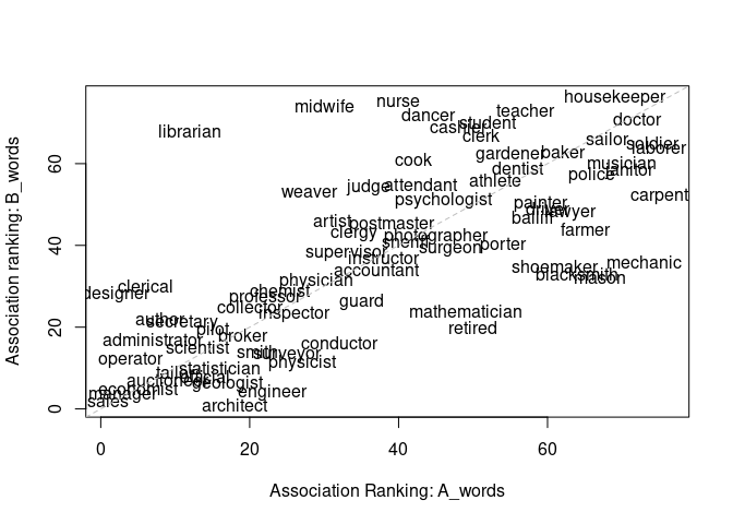
Effect size can also be calculated. It is the Spearman Correlation Coefficient of the two rows in P. Higher value indicates more “coherent”, i.e. less bias.
res
#>
#> ── sweater object ──────────────────────────────────────────────────────────────
#> Test type:  ect
#> Effect size:  0.7001504
#>
#> ── Functions ───────────────────────────────────────────────────────────────────
#> • `calculate_es()`: Calculate effect size
#> • `plot()`: Plot the bias of each individual word
Example: Relative Negative Sentiment Bias
This analysis attempts to reproduce the analysis in Sweeney & Najafian (2019).
Please note that the datasets glove_sweeney, bing_pos and bing_neg are not included in the package. If you are interested in reproducing the analysis, the 3 datasets are available from here.
load("tests/testdata/bing_neg.rda")
load("tests/testdata/bing_pos.rda")
load("tests/testdata/glove_sweeney.rda")

S3 <- c("swedish", "irish", "mexican", "chinese", "filipino",
        "german", "english", "french", "norwegian", "american",
        "indian", "dutch", "russian", "scottish", "italian")
sn <- query(glove_sweeney, S_words = S3, A_words = bing_pos, B_words = bing_neg, method = "rnsb")
The analysis shows that indian, mexican, and russian are more likely to be associated with negative sentiment.
plot(sn)
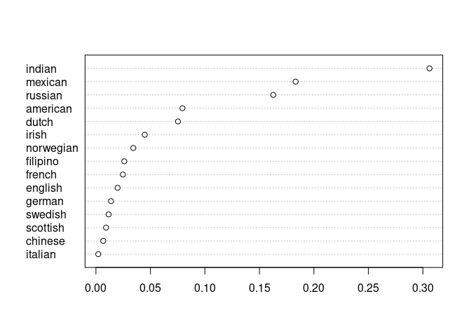
The effect size from the analysis is the Kullback–Leibler divergence of P from the uniform distribution. It is extremely close to the value reported in the original paper (0.6225).
sn
#>
#> ── sweater object ──────────────────────────────────────────────────────────────
#> Test type:  rnsb
#> Effect size:  0.6228853
#>
#> ── Functions ───────────────────────────────────────────────────────────────────
#> • `calculate_es()`: Calculate effect size
#> • `plot()`: Plot the bias of each individual word
Support for Quanteda Dictionaries
rnsb supports quanteda dictionaries as S_words. This support will be expanded to other methods later.
This analysis uses the data from here.
For example, newsmap_europe is an abridged dictionary from the package newsmap (Watanabe, 2018). The dictionary contains keywords of European countries and has two levels: regional level (e.g. Eastern Europe) and country level (e.g. Germany).
load("tests/testdata/newsmap_europe.rda")
load("tests/testdata/dictionary_demo.rda")

require(quanteda)
#> Loading required package: quanteda
#> Package version: 3.3.1
#> Unicode version: 14.0
#> ICU version: 70.1
#> Parallel computing: 8 of 8 threads used.
#> See https://quanteda.io for tutorials and examples.
newsmap_europe
#> Dictionary object with 4 primary key entries and 2 nested levels.
#> - [EAST]:
#>   - [BG]:
#>     - bulgaria, bulgarian*, sofia
#>   - [BY]:
#>     - belarus, belarusian*, minsk
#>   - [CZ]:
#>     - czech republic, czech*, prague
#>   - [HU]:
#>     - hungary, hungarian*, budapest
#>   - [MD]:
#>     - moldova, moldovan*, chisinau
#>   - [PL]:
#>     - poland, polish, pole*, warsaw
#>   [ reached max_nkey ... 4 more keys ]
#> - [NORTH]:
#>   - [AX]:
#>     - aland islands, aland island*, alandish, mariehamn
#>   - [DK]:
#>     - denmark, danish, dane*, copenhagen
#>   - [EE]:
#>     - estonia, estonian*, tallinn
#>   - [FI]:
#>     - finland, finnish, finn*, helsinki
#>   - [FO]:
#>     - faeroe islands, faeroe island*, faroese*, torshavn
#>   - [GB]:
#>     - uk, united kingdom, britain, british, briton*, brit*, london
#>   [ reached max_nkey ... 10 more keys ]
#> - [SOUTH]:
#>   - [AD]:
#>     - andorra, andorran*
#>   - [AL]:
#>     - albania, albanian*, tirana
#>   - [BA]:
#>     - bosnia, bosnian*, bosnia and herzegovina, herzegovina, sarajevo
#>   - [ES]:
#>     - spain, spanish, spaniard*, madrid, barcelona
#>   - [GI]:
#>     - gibraltar, gibraltarian*, llanitos
#>   - [GR]:
#>     - greece, greek*, athens
#>   [ reached max_nkey ... 11 more keys ]
#> - [WEST]:
#>   - [AT]:
#>     - austria, austrian*, vienna
#>   - [BE]:
#>     - belgium, belgian*, brussels
#>   - [CH]:
#>     - switzerland, swiss*, zurich, bern
#>   - [DE]:
#>     - germany, german*, berlin, frankfurt
#>   - [FR]:
#>     - france, french*, paris
#>   - [LI]:
#>     - liechtenstein, liechtenstein*, vaduz
#>   [ reached max_nkey ... 3 more keys ]
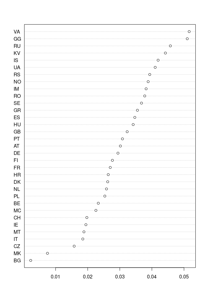
Country-level analysis
country_level <- rnsb(w = dictionary_demo, S_words = newsmap_europe, A_words = bing_pos, B_words = bing_neg, levels = 2)
plot(country_level)
Region-level analysis
region_level <- rnsb(w = dictionary_demo, S_words = newsmap_europe, A_words = bing_pos, B_words = bing_neg, levels = 1)
plot(region_level)
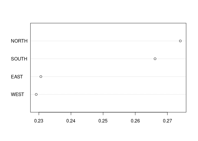
Comparison of the two effect sizes. Please note the much smaller effect size from region-level analysis. It reflects the evener distribution of P across regions than across countries.
calculate_es(country_level)
#> [1] 0.0796689
calculate_es(region_level)
#> [1] 0.00329434
Example: Normalized Association Score
Normalized Association Score (Caliskan et al., 2017) is similar to Relative Norm Distance above. It was used in Müller et al. (2023).
S3 <- c("janitor", "statistician", "midwife", "bailiff", "auctioneer",
"photographer", "geologist", "shoemaker", "athlete", "cashier",
"dancer", "housekeeper", "accountant", "physicist", "gardener",
"dentist", "weaver", "blacksmith", "psychologist", "supervisor",
"mathematician", "surveyor", "tailor", "designer", "economist",
"mechanic", "laborer", "postmaster", "broker", "chemist", "librarian",
"attendant", "clerical", "musician", "porter", "scientist", "carpenter",
"sailor", "instructor", "sheriff", "pilot", "inspector", "mason",
"baker", "administrator", "architect", "collector", "operator",
"surgeon", "driver", "painter", "conductor", "nurse", "cook",
"engineer", "retired", "sales", "lawyer", "clergy", "physician",
"farmer", "clerk", "manager", "guard", "artist", "smith", "official",
"police", "doctor", "professor", "student", "judge", "teacher",
"author", "secretary", "soldier")
A3 <- c("he", "son", "his", "him", "father", "man", "boy", "himself",
"male", "brother", "sons", "fathers", "men", "boys", "males",
"brothers", "uncle", "uncles", "nephew", "nephews")
B3 <- c("she", "daughter", "hers", "her", "mother", "woman", "girl",
"herself", "female", "sister", "daughters", "mothers", "women",
"girls", "females", "sisters", "aunt", "aunts", "niece", "nieces"
)

nas_f1 <- query(googlenews, S_words= S3, A_words = A3, B_words = B3, method = "nas")
plot(nas_f1)
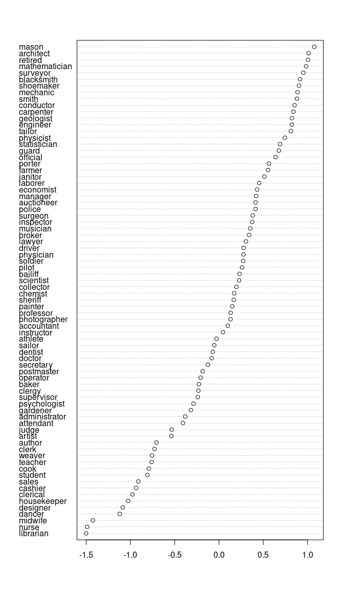
There is a very strong correlation between NAS and RND.
cor.test(nas_f1$P, garg_f1$P)
#>
#>  Pearson's product-moment correlation
#>
#> data:  nas_f1$P and garg_f1$P
#> t = -24.93, df = 74, p-value < 2.2e-16
#> alternative hypothesis: true correlation is not equal to 0
#> 95 percent confidence interval:
#>  -0.9650781 -0.9148179
#> sample estimates:
#>        cor
#> -0.9453038
Example: Word Embedding Association Test
This example reproduces the detection of “Math. vs Arts” gender bias in Caliskan et al (2017).
data(glove_math) # a subset of the original GLoVE word vectors

S4 <- c("math", "algebra", "geometry", "calculus", "equations", "computation", "numbers", "addition")
T4 <- c("poetry", "art", "dance", "literature", "novel", "symphony", "drama", "sculpture")
A4 <- c("male", "man", "boy", "brother", "he", "him", "his", "son")
B4 <- c("female", "woman", "girl", "sister", "she", "her", "hers", "daughter")
sw <- query(glove_math, S4, T4, A4, B4)

# extraction of effect size
sw
#>
#> ── sweater object ──────────────────────────────────────────────────────────────
#> Test type:  weat
#> Effect size:  1.055015
#>
#> ── Functions ───────────────────────────────────────────────────────────────────
#> • `calculate_es()`: Calculate effect size
#> • `weat_resampling()`: Conduct statistical test
A note about the effect size
By default, the effect size from the function weat_es is adjusted by the pooled standard deviaion (see Page 2 of Caliskan et al. 2007). The standardized effect size can be interpreted the way as Cohen’s d (Cohen, 1988).
One can also get the unstandardized version (aka. test statistic in the original paper):
## weat_es
calculate_es(sw, standardize = FALSE)
#> [1] 0.02486533
The original implementation assumes equal size of S and T. This assumption can be relaxed by pooling the standard deviaion with sample size adjustment. The function weat_es does it when S and T are of different length.
Also, the effect size can be converted to point-biserial correlation (mathematically equivalent to the Pearson’s product moment correlation).
weat_es(sw, r = TRUE)
#> [1] 0.4912066
Exact test
The exact test described in Caliskan et al. (2017) is also available. But it takes a long time to calculate.
## Don't do it. It takes a long time and is almost always significant.
weat_exact(sw)
Instead, please use the resampling approximation of the exact test. The p-value is very close to the reported 0.018.
weat_resampling(sw)
#>
#>  Resampling approximation of the exact test in Caliskan et al. (2017)
#>
#> data:  sw
#> bias = 0.024865, p-value = 0.0171
#> alternative hypothesis: true bias is greater than 7.245425e-05
#> sample estimates:
#>       bias
#> 0.02486533
How to get help
- Read the documentation
- Search for issues
Contributing
Contributions in the form of feedback, comments, code, and bug report are welcome.
- Fork the source code, modify, and issue a pull request.
- Issues, bug reports: File a Github issue.
Code of Conduct
Please note that the sweater project is released with a Contributor Code of Conduct. By contributing to this project, you agree to abide by its terms.
References
- An, J., Kwak, H., & Ahn, Y. Y. (2018). SemAxis: A lightweight framework to characterize domain-specific word semantics beyond sentiment. arXiv preprint arXiv:1806.05521.
- Badilla, P., Bravo-Marquez, F., & Pérez, J. (2020). WEFE: The word embeddings fairness evaluation framework. In Proceedings of the 29 th Intern. Joint Conf. Artificial Intelligence.
- Brunet, M. E., Alkalay-Houlihan, C., Anderson, A., & Zemel, R. (2019, May). Understanding the origins of bias in word embeddings. In International Conference on Machine Learning (pp. 803-811). PMLR.
- Caliskan, Aylin, Joanna J. Bryson, and Arvind Narayanan. “Semantics derived automatically from language corpora contain human-like biases.” Science 356.6334 (2017): 183-186.
- Cohen, J. (1988), Statistical Power Analysis for the Behavioral Sciences, 2nd Edition. Hillsdale: Lawrence Erlbaum.
- Dev, S., & Phillips, J. (2019, April). Attenuating bias in word vectors. In The 22nd International Conference on Artificial Intelligence and Statistics (pp. 879-887). PMLR.
- Garg, N., Schiebinger, L., Jurafsky, D., & Zou, J. (2018). Word embeddings quantify 100 years of gender and ethnic stereotypes. Proceedings of the National Academy of Sciences, 115(16), E3635-E3644.
- Manzini, T., Lim, Y. C., Tsvetkov, Y., & Black, A. W. (2019). Black is to criminal as caucasian is to police: Detecting and removing multiclass bias in word embeddings. arXiv preprint arXiv:1904.04047.
- McGrath, R. E., & Meyer, G. J. (2006). When effect sizes disagree: the case of r and d. Psychological methods, 11(4), 386.
- Müller, P., Chan, C. H., Ludwig, K., Freudenthaler, R., & Wessler, H. (2023). Differential Racism in the News: Using Semi-Supervised Machine Learning to Distinguish Explicit and Implicit Stigmatization of Ethnic and Religious Groups in Journalistic Discourse. Political Communication, 1-19.
- Rosenthal, R. (1991), Meta-Analytic Procedures for Social Research. Newbury Park: Sage
- Sweeney, C., & Najafian, M. (2019, July). A transparent framework for evaluating unintended demographic bias in word embeddings. In Proceedings of the 57th Annual Meeting of the Association for Computational Linguistics (pp. 1662-1667).
- Watanabe, K. (2018). Newsmap: A semi-supervised approach to geographical news classification. Digital Journalism, 6(3), 294-309.
In the pre 0.1.0 version of this package, the package used
S,T,A, andBas the main parameters. It was later rejected because the symbolTis hardlinked to the logical valueTRUEas a global variable; and it is considered to be a bad style to use the symbolT. Accordingly, they were renamed toS_words,T_words,A_words, andB_wordsrespectively. But in general, please stop using the symbolTto representTRUE!Please use the
queryfunction. These functions are kept for backward compatibility.