Stagewise Variable Selection for Joint Models of Semi-Competing Risks.
- swjm: Stagewise Variable Selection for Joint Models of Semi-Competing Risks
- Overview
- Installation
- Data format
- Workflow
- 1. Simulate data
- 2. Fit the stagewise regularization path
- 3. Plot the coefficient path
- 4. Cross-validation to select the tuning parameter
- 5. Plot the cross-validation results
- 6. Summarize the chosen model
- 7. Baseline hazard
- 8. Predict survival curves
- 9. Plot survival curves and predictor contributions
- 10. JSCM workflow (cross-validation + survival prediction)
- 11. Other penalties
- 12. Model evaluation
- Package conventions
swjm: Stagewise Variable Selection for Joint Models of Semi-Competing Risks
Overview
swjm implements stagewise (forward-stepwise) variable selection for joint models of recurrent events and terminal events (semi-competing risks). Two model frameworks are supported:
| Model | Type | alpha (first p) | beta (second p) |
|---|---|---|---|
| JFM | Cox frailty | recurrence/readmission | terminal/death |
| JSCM | Scale-change (AFT) | recurrence/readmission | terminal/death |
Three penalty types are available: cooperative lasso ("coop"), lasso ("lasso"), and group lasso ("group"). The cooperative lasso encourages shared support between the readmission and death coefficient vectors.
Installation
# From the package directory:
devtools::install("swjm")
Data format
All functions expect a data frame with columns id, t.start, t.stop, event (1 = readmission, 0 = terminal/censoring row), status (1 = death, 0 = alive/censored), and covariate columns x1, ..., xp.
Workflow
1. Simulate data
library(swjm)

# Joint Frailty Model — scenario 1
set.seed(42)
dat_jfm  <- generate_data(n = 200, p = 100, scenario = 1, model = "jfm")
Data_jfm <- dat_jfm$data

# JSCM — same scenario
set.seed(42)
dat_jscm  <- generate_data(n = 200, p = 100, scenario = 1, model = "jscm")
#> Call:
#> reReg::simGSC(n = n, summary = TRUE, para = para, xmat = X, censoring = C,
#>     frailty = gamma, tau = 60)
#>
#> Summary:
#> Sample size:                                    200
#> Number of recurrent event observed:             343
#> Average number of recurrent event per subject:  1.715
#> Proportion of subjects with a terminal event:   0.175
Data_jscm <- dat_jscm$data
JFM data: n = 200 subjects, 382 readmission events, 48 deaths
2. Fit the stagewise regularization path
fit_jfm <- stagewise_fit(Data_jfm, model = "jfm", penalty = "coop")
fit_jfm
#> Stagewise path (jfm/coop)
#>
#>   Covariates (p):            100
#>   Iterations:                5000
#>   Lambda range:              [0.08902, 1.301]
#>   Active at final step:      44 readmission, 34 death
#>     Readmission (alpha): 1, 2, 3, 4, 5, 7, 9, 10, 12, 14, 15, 17, 23, 33, 35, 37, 38, 39, 41, 43, 47, 49, 52, 55, 57, 60, 62, 64, 66, 67, 69, 71, 73, 74, 77, 79, 80, 82, 92, 93, 95, 96, 97, 98
#>     Death (beta):        3, 4, 5, 7, 9, 10, 12, 14, 15, 17, 25, 37, 38, 39, 41, 43, 47, 49, 52, 57, 60, 62, 66, 67, 73, 74, 78, 80, 82, 84, 95, 96, 97, 98
The fit object now exposes alpha (readmission) and beta (death) as separate p × (k+1) matrices — one column per stagewise step — in addition to the combined theta matrix (2p × (k+1)):
p <- 100
k_final <- ncol(fit_jfm$alpha)
a_final <- round(fit_jfm$alpha[, k_final], 4)
- alpha matrix: 100 rows x 5001 columns
- beta matrix: 100 rows x 5001 columns
Nonzero alpha entries at final step:
a_final[a_final != 0]
#>  [1]  1.0057 -0.9787  0.0183 -0.0577  0.0185  0.0151  0.9614 -0.8484  0.0124
#> [10]  0.0423 -0.0284  0.0199 -0.0020  0.0240 -0.0240  0.0064  0.0781 -0.0061
#> [19]  0.0125  0.0046 -0.0429  0.0396  0.0092  0.0680 -0.0550 -0.0500 -0.0007
#> [28]  0.0200  0.0742  0.0005 -0.0350  0.0370  0.0099 -0.0234  0.0450  0.0790
#> [37] -0.0072  0.0013 -0.0200  0.0150  0.0085  0.0027 -0.0618  0.0272
summary() shows a compact table of path-end coefficients with variable type (shared, readmission-only, or death-only):
summary(fit_jfm)
#> Stagewise path (jfm/coop)
#>
#>   p = 100  |  5000 iterations  |  lambda: [0.08902, 1.301]
#>   Decreasing path: 784 steps
#>
#>   Path-end coefficients (nonzero variables):
#>
#>   Variable    alpha       beta        Type
#>   ----------  ----------  ----------  ----------------
#>   x9          +0.9614     +0.6629     shared (+)
#>   x4          -0.0577     -0.9979     shared (+)
#>   x10         -0.8484     -0.7274     shared (+)
#>   x2          -0.9787          —    readmission only
#>   x3          +0.0183     +0.8049     shared (+)
#>   x74         -0.0234     -0.3101     shared (+)
#>   x1          +1.0057          —    readmission only
#>   x67         +0.0005     +0.1393     shared (+)
#>   x57         -0.0550     +0.1330     shared (–)
#>   x38         +0.0781     +0.0857     shared (+)
#>   x97         -0.0618     -0.0583     shared (+)
#>   x66         +0.0742     +0.0415     shared (+)
#>   x41         +0.0125     +0.0937     shared (+)
#>   x55         +0.0680          —    readmission only
#>   x79         +0.0790          —    readmission only
#>   x60         -0.0500     +0.0070     shared (–)
#>   x49         +0.0396     +0.0305     shared (+)
#>   x98         +0.0272     +0.0792     shared (+)
#>   x15         -0.0284     -0.0639     shared (+)
#>   x7          +0.0151     +0.1160     shared (+)
#>   x82         +0.0013     +0.0750     shared (+)
#>   x5          +0.0185     +0.0527     shared (+)
#>   x39         -0.0061     -0.0657     shared (+)
#>   x14         +0.0423     +0.0076     shared (+)
#>   x47         -0.0429     -0.0135     shared (+)
#>   x71         +0.0370          —    readmission only
#>   x77         +0.0450          —    readmission only
#>   x69         -0.0350          —    readmission only
#>   x35         -0.0240          —    readmission only
#>   x33         +0.0240          —    readmission only
#>   x17         +0.0199     +0.0020     shared (+)
#>   x84              —    -0.0790     death only
#>   x37         +0.0064     +0.0394     shared (+)
#>   x78              —    +0.0710     death only
#>   x64         +0.0200          —    readmission only
#>   x92         -0.0200          —    readmission only
#>   x25              —    +0.0200     death only
#>   x80         -0.0072     -0.0165     shared (+)
#>   x93         +0.0150          —    readmission only
#>   x12         +0.0124     +0.0085     shared (+)
#>   x73         +0.0099     +0.0084     shared (+)
#>   x95         +0.0085     +0.0170     shared (+)
#>   x52         +0.0092     +0.0092     shared (+)
#>   x43         +0.0046     +0.0038     shared (+)
#>   x96         +0.0027     +0.0054     shared (+)
#>   x23         -0.0020          —    readmission only
#>   x62         -0.0007     -0.0007     shared (+)
#>
#>   Inactive: x6, x8, x11, x13, x16, x18, x19, x20, x21, x22, x24, x26, x27, x28, x29, x30, x31, x32, x34, x36, x40, x42, x44, x45, x46, x48, x50, x51, x53, x54, x56, x58, x59, x61, x63, x65, x68, x70, x72, x75, x76, x81, x83, x85, x86, x87, x88, x89, x90, x91, x94, x99, x100
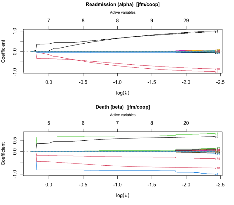
3. Plot the coefficient path
plot() produces a glmnet-style coefficient trajectory plot with the number of active variables on the top axis:
plot(fit_jfm)
4. Cross-validation to select the tuning parameter
cv_stagewise() evaluates a cross-fitted estimating-equation score norm over a grid of lambda values.
lambda_path <- fit_jfm$lambda
dec_idx     <- swjm:::extract_decreasing_indices(lambda_path)
lambda_seq  <- lambda_path[dec_idx]

cv_jfm <- cv_stagewise(
  Data_jfm, model = "jfm", penalty = "coop",
  lambda_seq = lambda_seq, K = 3L
)
cv_jfm
#> Cross-validation (jfm/coop)
#>
#>   Covariates (p):              100
#>   Lambda grid size:            784
#>   Best position (combined):    438  (lambda = 0.9241)
#>   Selected variables:          8 readmission, 6 death
#>     Readmission (alpha): 1, 2, 3, 4, 9, 10, 67, 74
#>     Death (beta):        3, 4, 9, 10, 67, 74
The CV object stores alpha and beta at the optimal lambda, plus n_active_alpha, n_active_beta, and n_active variable-count vectors across the full lambda grid.
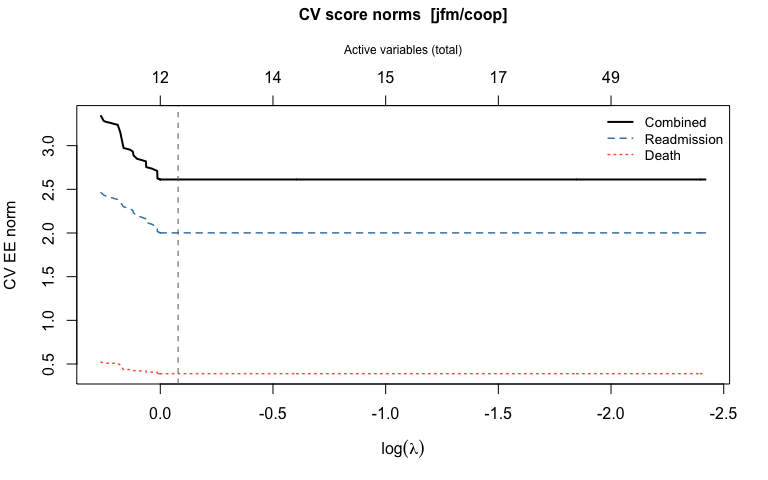
5. Plot the cross-validation results
plot(cv_jfm)
6. Summarize the chosen model
# summary() shows a formatted table of selected coefficients
summary(cv_jfm)
#> CV-selected model (jfm/coop)
#>
#>   p = 100  |  Lambda grid: 784 steps  |  CV optimal: step 438 (lambda = 0.9241)
#>
#>   Selected coefficients  (8 readmission, 6 death):
#>
#>   Variable    alpha       beta        Type
#>   ----------  ----------  ----------  ----------------
#>   x9          +0.4338     +0.4528     shared (+)
#>   x4          -0.0466     -0.8184     shared (+)
#>   x10         -0.3531     -0.4622     shared (+)
#>   x3          +0.0075     +0.6503     shared (+)
#>   x2          -0.2507          —    readmission only
#>   x74         -0.0162     -0.1793     shared (+)
#>   x1          +0.1597          —    readmission only
#>   x67         +0.0004     +0.0133     shared (+)
#>
#>   Inactive (92): x5, x6, x7, x8, x11, x12, x13, x14, x15, x16, x17, x18, x19, x20, x21, x22, x23, x24, x25, x26, x27, x28, x29, x30, x31, x32, x33, x34, x35, x36, x37, x38, x39, x40, x41, x42, x43, x44, x45, x46, x47, x48, x49, x50, x51, x52, x53, x54, x55, x56, x57, x58, x59, x60, x61, x62, x63, x64, x65, x66, x68, x69, x70, x71, x72, x73, x75, x76, x77, x78, x79, x80, x81, x82, x83, x84, x85, x86, x87, x88, x89, x90, x91, x92, x93, x94, x95, x96, x97, x98, x99, x100
Direct access to selected coefficients:
# coef() returns the combined numeric vector c(alpha, beta) for compatibility
theta_best <- coef(cv_jfm)
- Selected readmission (alpha) variables: 1 2 3 4 9 10 67 74
- Selected death (beta) variables: 3 4 9 10 67 74
7. Baseline hazard
baseline_hazard() evaluates the cumulative baseline hazards at any desired time points (Breslow for JFM; Nelson-Aalen on the accelerated scale for JSCM):
bh <- baseline_hazard(cv_jfm, times = c(0.5, 1.0, 2.0, 4.0, 6.0))
print(bh)
#>   time cumhaz_readmission cumhaz_death
#> 1  0.5          0.8302786   0.04821411
#> 2  1.0          1.3776457   0.06859515
#> 3  2.0          1.9078200   0.12461276
#> 4  4.0          3.1933429   0.28725353
#> 5  6.0          4.5481622   0.33588232
8. Predict survival curves
predict() computes subject-specific readmission-free and death-free survival curves, together with the per-predictor contributions to each linear predictor:
# Three hypothetical new subjects (covariate vectors of length p = 100)
set.seed(7)
newz <- matrix(rnorm(300), nrow = 3, ncol = 100)
colnames(newz) <- paste0("x", 1:100)

pred <- predict(cv_jfm, newdata = newz)
pred
#> swjm predictions (jfm)
#>
#>   Subjects:                3
#>   Time points:             430
#>   Time range:              [0.0002844, 6.281]
#>
#>   Use plot() to visualize survival curves and predictor contributions.

# S_re: readmission-free survival — first 10 time points
round(pred$S_re[, 1:10], 3)
#>          t=0.0002844 t=0.0009392 t=0.001171 t=0.001381 t=0.001936 t=0.002432
#> Subject1       0.992       0.983      0.983      0.974      0.966      0.957
#> Subject2       0.994       0.987      0.987      0.980      0.973      0.967
#> Subject3       0.994       0.987      0.987      0.981      0.974      0.967
#>          t=0.004535 t=0.004809 t=0.006178 t=0.006205
#> Subject1      0.949      0.940      0.932      0.923
#> Subject2      0.960      0.953      0.947      0.940
#> Subject3      0.961      0.954      0.948      0.941

# Predictor contributions for subject 1 — show only nonzero entries
contrib1 <- round(pred$contrib_re[1, ], 3)
contrib1[contrib1 != 0]
#>     x1     x2     x3     x4     x9    x10    x74
#>  0.365  0.103  0.006 -0.102  0.552 -0.209  0.007
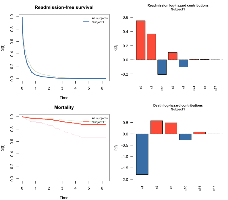
9. Plot survival curves and predictor contributions
plot() on a swjm_pred object draws four panels: survival curves for both processes (all subjects in grey, highlighted subject in color) plus bar charts of predictor contributions for the selected subject.
plot(pred, which_subject = 1)
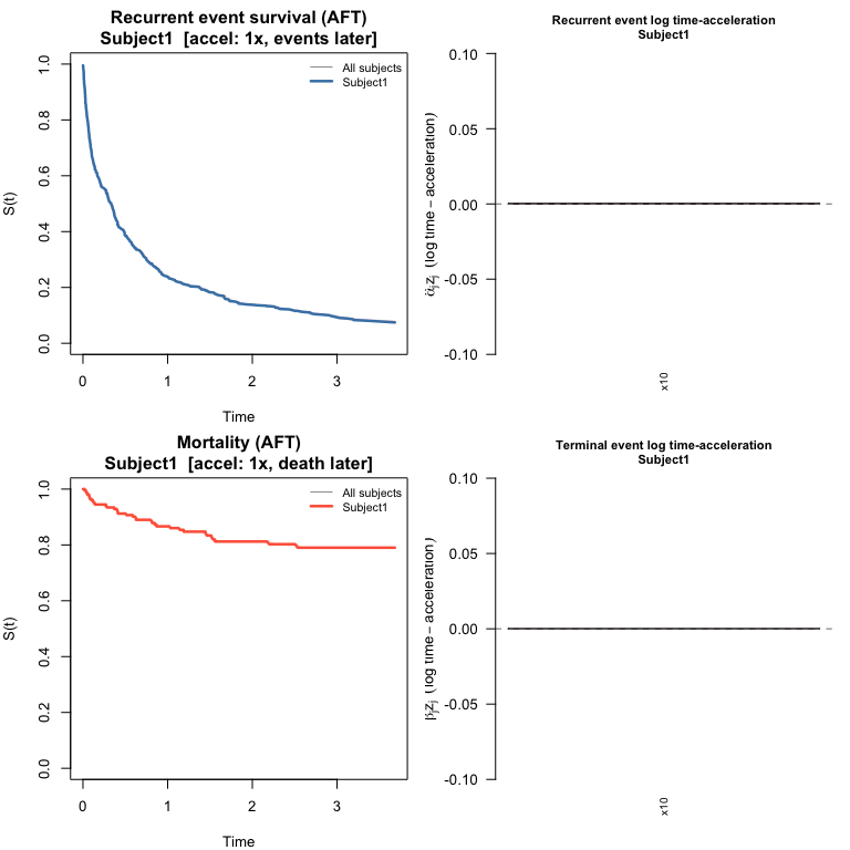
10. JSCM workflow (cross-validation + survival prediction)
The same workflow applies to the JSCM. baseline_hazard() and predict() now work for both models: for JSCM, survival curves are estimated via a Nelson-Aalen baseline on the accelerated time scale. In the AFT interpretation, $e^{\hat\alpha^\top z_i}$ is the time-acceleration factor for subject $i$: greater than 1 means events happen sooner, less than 1 means later.
fit_jscm <- stagewise_fit(Data_jscm, model = "jscm", penalty = "coop")

lambda_path_jscm <- fit_jscm$lambda
dec_idx_jscm     <- swjm:::extract_decreasing_indices(lambda_path_jscm)
lambda_seq_jscm  <- lambda_path_jscm[dec_idx_jscm]

cv_jscm <- cv_stagewise(
  Data_jscm, model = "jscm", penalty = "coop",
  lambda_seq = lambda_seq_jscm, K = 3L
)
summary(cv_jscm)
#> CV-selected model (jscm/coop)
#>
#>   p = 100  |  Lambda grid: 30 steps  |  CV optimal: step 3 (lambda = 0.6838)
#>
#>   Selected coefficients  (1 readmission, 1 death):
#>
#>   Variable    alpha       beta        Type
#>   ----------  ----------  ----------  ----------------
#>   x10         -0.0180     -0.0088     shared (+)
#>
#>   Inactive (99): x1, x2, x3, x4, x5, x6, x7, x8, x9, x11, x12, x13, x14, x15, x16, x17, x18, x19, x20, x21, x22, x23, x24, x25, x26, x27, x28, x29, x30, x31, x32, x33, x34, x35, x36, x37, x38, x39, x40, x41, x42, x43, x44, x45, x46, x47, x48, x49, x50, x51, x52, x53, x54, x55, x56, x57, x58, x59, x60, x61, x62, x63, x64, x65, x66, x67, x68, x69, x70, x71, x72, x73, x74, x75, x76, x77, x78, x79, x80, x81, x82, x83, x84, x85, x86, x87, x88, x89, x90, x91, x92, x93, x94, x95, x96, x97, x98, x99, x100
set.seed(7)
newz_jscm <- matrix(runif(600, -1, 1), nrow = 3, ncol = 100)
#> Warning in matrix(runif(600, -1, 1), nrow = 3, ncol = 100): data length differs
#> from size of matrix: [600 != 3 x 100]

pred_jscm <- predict(cv_jscm, newdata = newz_jscm)
Recurrence time-acceleration factors:
round(pred_jscm$time_accel_re, 3)
#> Subject1 Subject2 Subject3
#>    1.000    0.983    1.005
plot() draws the same four-panel layout as for JFM: survival curves for both processes plus bar charts of log time-acceleration contributions.
plot(pred_jscm, which_subject = 1)
11. Other penalties
fit_lasso <- stagewise_fit(Data_jfm, model = "jfm", penalty = "lasso")
cv_lasso  <- cv_stagewise(Data_jfm, model = "jfm", penalty = "lasso", K = 3L)
summary(cv_lasso)

fit_group <- stagewise_fit(Data_jfm, model = "jfm", penalty = "group")
cv_group  <- cv_stagewise(Data_jfm, model = "jfm", penalty = "group", K = 3L)
summary(cv_group)
12. Model evaluation
12.1 Coefficient recovery
Compare CV-optimal estimates to the true generating coefficients. Variables that are truly nonzero or were selected are shown; all others were correctly excluded.
p <- 100

# JFM: variables of interest (true signal or selected)
show_jfm <- sort(which(dat_jfm$alpha_true != 0 | cv_jfm$alpha != 0 |
                       dat_jfm$beta_true  != 0 | cv_jfm$beta  != 0))

coef_df <- data.frame(
  variable   = paste0("x", show_jfm),
  true_alpha = round(dat_jfm$alpha_true[show_jfm], 3),
  est_alpha  = round(cv_jfm$alpha[show_jfm],       3),
  true_beta  = round(dat_jfm$beta_true[show_jfm],  3),
  est_beta   = round(cv_jfm$beta[show_jfm],        3)
)
colnames(coef_df) <- c("variable", "alpha_true", "alpha_est", "beta_true", "beta_est")
print(coef_df, row.names = FALSE)
#>  variable alpha_true alpha_est beta_true beta_est
#>        x1        1.1     0.160       0.1    0.000
#>        x2       -1.1    -0.251      -0.1    0.000
#>        x3        0.1     0.007       1.1    0.650
#>        x4       -0.1    -0.047      -1.1   -0.818
#>        x9        1.0     0.434       1.0    0.453
#>       x10       -1.0    -0.353      -1.0   -0.462
#>       x67        0.0     0.000       0.0    0.013
#>       x74        0.0    -0.016       0.0   -0.179
JFM alpha: TP=6 FP=2 FN=0 | beta: TP=4 FP=2 FN=2
show_jscm <- sort(which(dat_jscm$alpha_true != 0 | cv_jscm$alpha != 0 |
                        dat_jscm$beta_true  != 0 | cv_jscm$beta  != 0))

coef_jscm <- data.frame(
  variable   = paste0("x", show_jscm),
  true_alpha = round(dat_jscm$alpha_true[show_jscm], 3),
  est_alpha  = round(cv_jscm$alpha[show_jscm],        3),
  true_beta  = round(dat_jscm$beta_true[show_jscm],  3),
  est_beta   = round(cv_jscm$beta[show_jscm],         3)
)
colnames(coef_jscm) <- c("variable", "alpha_true", "alpha_est", "beta_true", "beta_est")
print(coef_jscm, row.names = FALSE)
#>  variable alpha_true alpha_est beta_true beta_est
#>        x1        1.1     0.000       0.1    0.000
#>        x2       -1.1     0.000      -0.1    0.000
#>        x3        0.1     0.000       1.1    0.000
#>        x4       -0.1     0.000      -1.1    0.000
#>        x9        1.0     0.000       1.0    0.000
#>       x10       -1.0    -0.018      -1.0   -0.009
JSCM alpha: TP=1 FP=0 FN=5 | beta: TP=1 FP=0 FN=5
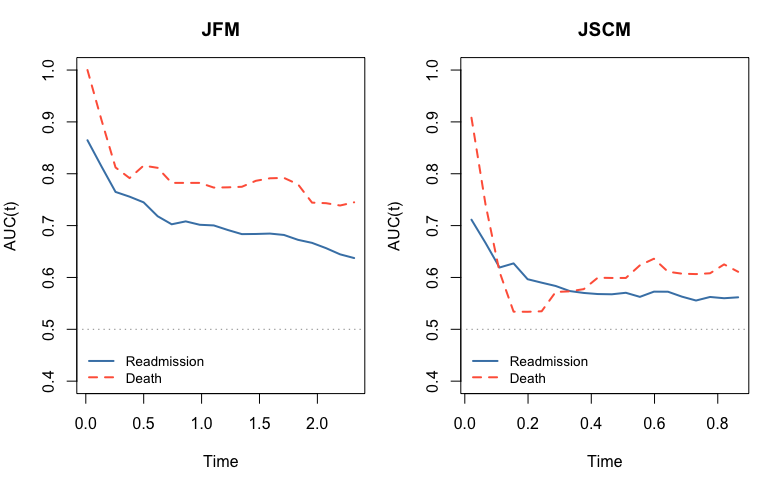
12.2 Time-varying AUC
We use the timeROC package (Blanche et al., 2013) to compute cause-specific time-varying AUC in the competing-risk framework. Each subject contributes at most a first-readmission event (cause 1) and a death event (cause 2). Each sub-model is assessed with its own linear predictor: $\hat\alpha^\top z_i$ for readmission, $\hat\beta^\top z_i$ for death.
Note: AUC is evaluated on the training data for illustration. In practice use held-out or cross-validated predictions.
# Construct competing-risk dataset:
# Keep first readmission (event==1 & t.start==0) + death/censor (event==0).
# Status: 1 = first readmission, 2 = death, 0 = censored.
.cr_data <- function(Data) {
  d3 <- Data[Data$event == 0 | (Data$event == 1 & Data$t.start == 0), ]
  d3 <- d3[order(d3$id, d3$t.start, d3$t.stop), ]
  status <- ifelse(d3$event == 1 & d3$status == 0, 1L,
             ifelse(d3$event == 0 & d3$status == 0, 0L, 2L))
  list(data = d3, status = status)
}

cr_jfm  <- .cr_data(Data_jfm)
cr_jscm <- .cr_data(Data_jscm)

# Baseline covariates (one row per subject)
Z_jfm  <- as.matrix(Data_jfm[!duplicated(Data_jfm$id),   paste0("x", 1:p)])
Z_jscm <- as.matrix(Data_jscm[!duplicated(Data_jscm$id), paste0("x", 1:p)])

# Markers expanded to row level: alpha^T z for readmission, beta^T z for death
M_re_jfm  <- drop(Z_jfm  %*% cv_jfm$alpha)[cr_jfm$data$id]
M_de_jfm  <- drop(Z_jfm  %*% cv_jfm$beta)[cr_jfm$data$id]
M_re_jscm <- drop(Z_jscm %*% cv_jscm$alpha)[cr_jscm$data$id]
M_de_jscm <- drop(Z_jscm %*% cv_jscm$beta)[cr_jscm$data$id]
if (!requireNamespace("timeROC", quietly = TRUE))
  install.packages("timeROC")
library(survival)
library(timeROC)

# Evaluation grid: 20 points spanning the 10th-85th percentile of event times
.tgrid <- function(t_vec, status, n = 20) {
  t_ev <- t_vec[status > 0]
  seq(quantile(t_ev, 0.10), quantile(t_ev, 0.85), length.out = n)
}

t_jfm  <- .tgrid(cr_jfm$data$t.stop,  cr_jfm$status)
t_jscm <- .tgrid(cr_jscm$data$t.stop, cr_jscm$status)

# Readmission AUC: alpha^T z marker, cause = 1
roc_re_jfm <- timeROC(T = cr_jfm$data$t.stop, delta = cr_jfm$status,
                       marker = M_re_jfm, cause = 1, weighting = "marginal",
                       times = t_jfm, ROC = FALSE, iid = FALSE)
roc_re_jscm <- timeROC(T = cr_jscm$data$t.stop, delta = cr_jscm$status,
                        marker = M_re_jscm, cause = 1, weighting = "marginal",
                        times = t_jscm, ROC = FALSE, iid = FALSE)

# Death AUC: beta^T z marker, cause = 2
roc_de_jfm <- timeROC(T = cr_jfm$data$t.stop, delta = cr_jfm$status,
                       marker = M_de_jfm, cause = 2, weighting = "marginal",
                       times = t_jfm, ROC = FALSE, iid = FALSE)
roc_de_jscm <- timeROC(T = cr_jscm$data$t.stop, delta = cr_jscm$status,
                        marker = M_de_jscm, cause = 2, weighting = "marginal",
                        times = t_jscm, ROC = FALSE, iid = FALSE)
.get_auc <- function(roc, cause) {
  auc <- roc[[paste0("AUC_", cause)]]
  if (is.null(auc)) auc <- roc$AUC
  if (is.null(auc) || !is.numeric(auc)) return(rep(NA_real_, length(roc$times)))
  if (length(auc) == length(roc$times) + 1) auc <- auc[-1]
  as.numeric(auc)
}

old_par <- par(mfrow = c(1, 2), mar = c(4.5, 4, 3, 1))

plot(t_jfm, .get_auc(roc_re_jfm, 1), type = "l", lwd = 2, col = "steelblue",
     xlab = "Time", ylab = "AUC(t)", main = "JFM", ylim = c(0.4, 1))
lines(t_jfm, .get_auc(roc_de_jfm, 2), lwd = 2, col = "tomato", lty = 2)
abline(h = 0.5, lty = 3, col = "grey60")
legend("bottomleft", c("Readmission", "Death"),
       col = c("steelblue", "tomato"), lwd = 2, lty = c(1, 2),
       bty = "n", cex = 0.85)

plot(t_jscm, .get_auc(roc_re_jscm, 1), type = "l", lwd = 2, col = "steelblue",
     xlab = "Time", ylab = "AUC(t)", main = "JSCM", ylim = c(0.4, 1))
lines(t_jscm, .get_auc(roc_de_jscm, 2), lwd = 2, col = "tomato", lty = 2)
abline(h = 0.5, lty = 3, col = "grey60")
legend("bottomleft", c("Readmission", "Death"),
       col = c("steelblue", "tomato"), lwd = 2, lty = c(1, 2),
       bty = "n", cex = 0.85)
par(old_par)
Package conventions
thetais always stored asc(alpha, beta):theta[1:p]=alpha(readmission),theta[(p+1):(2p)]=beta(death). This holds for both the JFM and JSCM.stagewise_fit()also returnsalphaandbetaas separate p × (k+1) matrices for convenient access to the full regularization path.cv_stagewise()storesalphaandbetaat the CV-optimal lambda, plus variable-count vectorsn_active_alpha,n_active_beta,n_active.- Baseline hazards: stored in
cv$baselineand accessible viabaseline_hazard(cv, times). Works for both models: Breslow estimator for JFM; Nelson-Aalen on the accelerated time scale for JSCM. Used internally bypredict(). - Survival prediction:
predict(cv, newdata)works for both models and returns aswjm_predobject withS_re,S_de(survival matrices), linear predictorslp_re,lp_de, and predictor-contribution matricescontrib_re,contrib_de($\hat\alpha_j z_{ij}$ and $\hat\beta_j z_{ij}$).- JFM: contributions are log-hazard-ratio contributions (positive = higher risk).
- JSCM: also returns
time_accel_reandtime_accel_de($e^{\hat\alpha^\top z_i}$, $e^{\hat\beta^\top z_i}$) — the multiplicative factors by which each subject’s event times are scaled relative to baseline. Contributions $\hat\alpha_j z_{ij}$ are log time-acceleration contributions: $e^{\hat\alpha_j z_{ij}} > 1$ shortens event times; $< 1$ lengthens them.
- The cooperative lasso norm penalizes each variable pair
(alpha_j, beta_j)with the L2 norm when signs agree, and L1 when they disagree — encouraging variables that affect both processes to enter together with the same sign. - Gradient scaling: at each step the death gradient is scaled up so that both sub-models contribute comparably to the penalty norm.
- Adaptive step size: the step size at each iteration is set to one order of magnitude smaller than the current dual norm, which avoids overly large updates.