Test (Multiple) Arguments of a User-Defined Prediction Algorithm.
testarguments
Prediction algorithms typically have at least one user-specified argument that can have a considerable effect on predictive performance. Specifying these arguments can be a tedious task, particularly if there is an interaction between argument levels. This package is designed to neatly and automatically test and visualise the performance of a user-defined prediction algorithm over an arbitrary number of arguments. It includes functions for testing the predictive performance of an algorithm with respect to a set of user-defined diagnostics, visualising the results of these tests, and finding the optimal argument combinations for each diagnostic. The typical workflow involves:
- Defining a prediction algorithm that uses training data and predicts over a testing set.
- Defining a set of diagnostics as a function that quantify the performance of the predictions over the testing set.
- Using
test_arguments()to train and test the prediction algorithm over a range of argument values. This creates an object of classtestargs, the central class definition of the package. - Visualising the predictive performance using
plot_diagnostics(). - Computing the optimal combination of arguments for each diagnostic using
optimal_arguments().
Example
Set up
We demonstrate the use of testarguments by predicting with the package FRK. First, load the required packages.
library("testarguments")
library("FRK")
library("sp")
library("pROC") # AUC score
Now create training and testing data.
n <- 5000                                                  # sample size
RNGversion("3.6.0"); set.seed(1)
data("MODIS_cloud_df") # MODIS dataframe stored in FRK (FRKTMB branch)
train_id <- sample(1:nrow(MODIS_cloud_df), n, replace = FALSE)
df_train <- MODIS_cloud_df[train_id, ]                     # training set
df_test  <- MODIS_cloud_df[-train_id, ]                    # testing set
Define a wrapper function which uses df_train to predict over df_test. This will be passed into test_arguments(). In this example, we wish to test values of link and nres, so we include these as arguments in the wrapper function.
pred_fun <- function(df_train, df_test, link, nres) {

  ## Convert dataframes to Spatial* objects (as required by FRK)
  coordinates(df_train) <- ~ x + y
  coordinates(df_test) <- ~ x + y

  ## BAUs (just use a grid over the spatial domain of interest)
  BAUs    <- SpatialPixelsDataFrame(points = expand.grid(x = 1:225, y = 1:150),
                                    data = expand.grid(x = 1:225, y = 1:150))

  ## Fit using df_train
  df_train$k_Z <- 1 # size parameter of the binomial distribution
  S <- FRK(f = z ~ 1, data = list(df_train), BAUs = BAUs, response = "binomial",
           link = link, nres = nres)

  ## Predict using df_test
  pred <- predict(S, newdata = df_test, type = "response")

  ## Returned object must be a matrix-like object with named columns
  return(pred$newdata@data)
}
Define diagnostic function: This should return a named vector.
diagnostic_fun <- function(df) {
  with(df, c(
    Brier = mean((z - p_Z)^2),
    AUC = as.numeric(pROC::auc(z, p_Z))
  ))
}
Test the arguments of the prediction algorithm
Compute the user-defined diagnostics over a range of arguments using test_arguments(). Here, we test the prediction algorithm with 1, 2, or 3 resolutions of basis functions, and using the logit or probit link function. This creates an object of class testargs.
testargs_object <- test_arguments(
  pred_fun, df_train, df_test, diagnostic_fun,
  arguments = list(link = c("logit", "probit"), nres = 1:3)
)
This produces an object of class testargs, the central class definition of the package testarguments.
Visualise predictive performance
Visualise the predictive performance across all argument combinations:
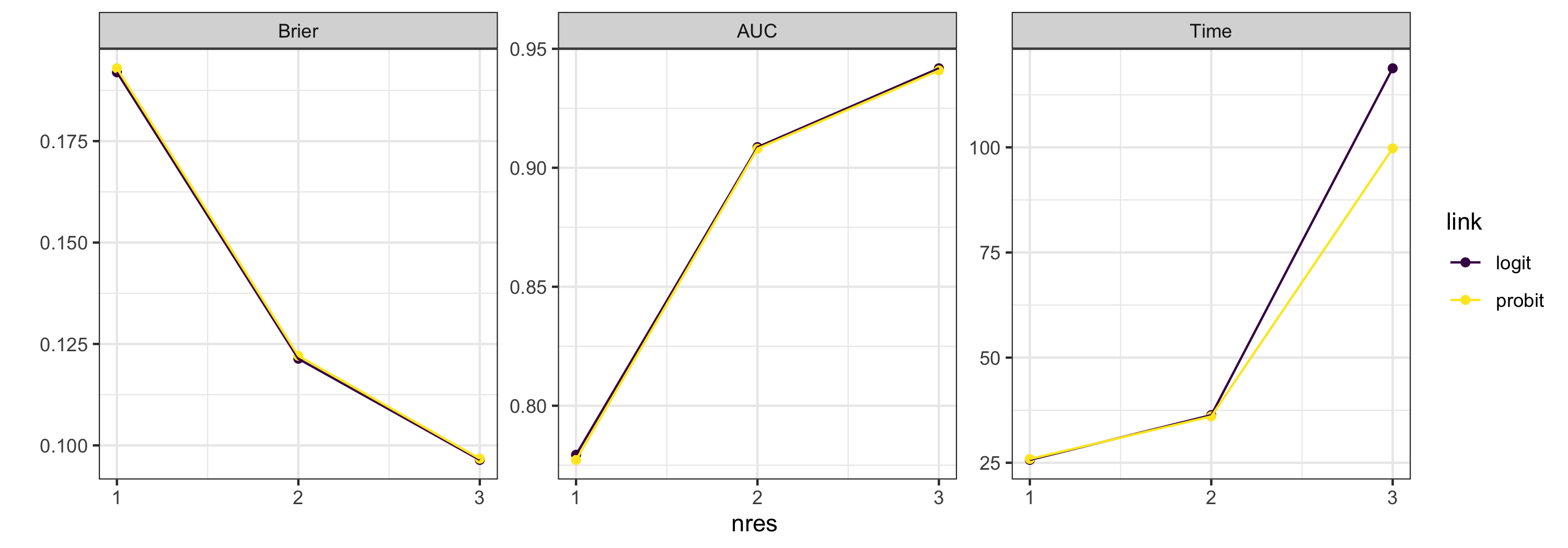
plot_diagnostics(testargs_object)

Using various aesthetics, plot_diagnostics() can visualise the performance of all combinations of up to 4 different arguments simultaneously. In the above plot, we can see that the predictive performance is not particularly sensitive to link function. We can focus on a subset of arguments using the argument focused_args. By default, this averages out the arguments which are not of interest.
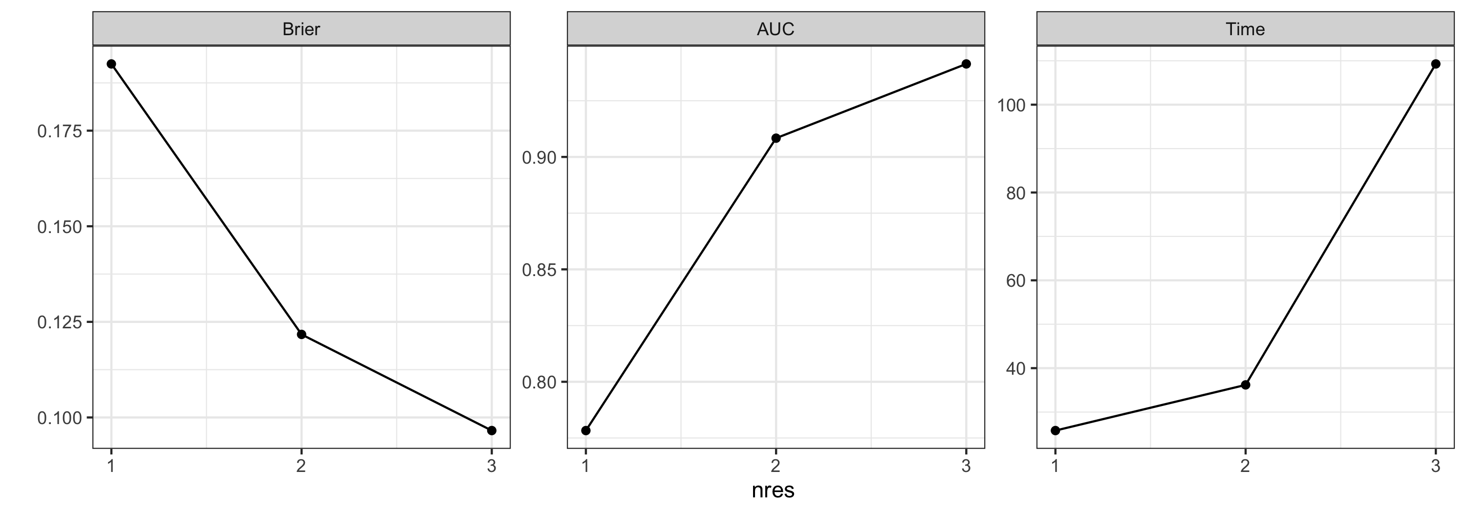
plot_diagnostics(testargs_object, focused_args = "nres")

Optimal arguments
The function optimal_arguments() computes the optimal arguments from a testargs object. The measure of optimality is diagnostic dependent (e.g., we wish to minimise the Brier score and run time, but maximise the AUC score). For this reason, optimal_arguments() allows one to set the optimality criterion for each rule individually. The default is to minimise.
optimality_criterion <- list(AUC = which.max)
optimal_arguments(testargs_object, optimality_criterion)
| which_diagnostic_optimal | Brier | AUC | Time | link | nres | |
|---|---|---|---|---|---|---|
| 1 | Brier | 0.10 | 0.94 | 94.83 | logit | 3 |
| 2 | AUC | 0.10 | 0.94 | 94.83 | logit | 3 |
| 3 | Time | 0.19 | 0.78 | 13.66 | probit | 1 |
More complicated criteria are possible: For instance, if one of the diagnostics is Cov90 (the coverage from 90% prediction intervals), then one would use something like list(Cov90 = function(x) which.min(abs(x - 0.90))).
Note that objects of class testargs can be combined using c().
Installation tips
To install testarguments, simply type the following command in R:
devtools::install_github("MattSainsbury-Dale/testarguments")