An R6 Class to Perform Analysis on Long Tidy Data.

tidymodlr

The goal of tidymodlr is to …

Installation

You can install the development version of tidymodlr from GitHub with:

# install.packages("devtools")
devtools::install_github("david-hammond/tidymodlr")

Example

This is a basic example which shows you how to solve a common problem with long data:

library(tidymodlr)
data(wb)
head(wb)
#> # A tibble: 6 × 4
#>   iso3c indicator          year    value
#>   <chr> <chr>             <dbl>    <dbl>
#> 1 DZA   Population, total  2012 37260563
#> 2 DZA   Population, total  2011 36543541
#> 3 DZA   Population, total  2010 35856344
#> 4 AGO   Population, total  2012 25188292
#> 5 AGO   Population, total  2011 24259111
#> 6 AGO   Population, total  2010 23364185

Here you can see that the format is not conducive to regression or other types of analysis that require wide formats. The indicator names are also long, making pivot_longer result in cumbersome column names. To assist, we build a tidymodl:

mdl <- tidymodl$new(wb,
                   pivot_column = "indicator",
                  pivot_value = "value")
print(mdl)
#> Key: 
#>   key                             indicator
#> 1 ein Energy imports, net (% of energy use)
#> 2 gcu                     GDP (current US$)
#> 3 gni                            Gini index
#> 4 icp Inflation, consumer prices (annual %)
#> 5 ppt                     Population, total
#> 6 trg                      Trade (% of GDP)
#> Matrix: 
#> # A tibble: 5 × 6
#>     ein           gcu   gni   icp      ppt   trg
#>   <dbl>         <dbl> <dbl> <dbl>    <dbl> <dbl>
#> 1 -213. 227143746076.  NA    8.89 37260563  60.8
#> 2 -249. 218331946925.  27.6  4.52 36543541  62.2
#> 3 -275. 177785053940.  NA    3.91 35856344  63.5
#> 4 -590. 128052915766.  NA   10.3  25188292  91.8
#> 5 -619. 111789747671.  NA   13.5  24259111 100.

This can now be used for regressions

### Use mdl$child for modelling
fit <- lm(data = mdl$child, gni ~ gcu + ppt)
summary(fit)
#> 
#> Call:
#> lm(formula = gni ~ gcu + ppt, data = mdl$child)
#> 
#> Residuals:
#>     Min      1Q  Median      3Q     Max 
#> -11.128  -5.515   1.219   4.132  24.701 
#> 
#> Coefficients:
#>               Estimate Std. Error t value Pr(>|t|)    
#> (Intercept)  3.959e+01  1.438e+00  27.523   <2e-16 ***
#> gcu          3.055e-12  9.031e-12   0.338    0.737    
#> ppt         -4.177e-08  3.828e-08  -1.091    0.282    
#> ---
#> Signif. codes:  0 '***' 0.001 '**' 0.01 '*' 0.05 '.' 0.1 ' ' 1
#> 
#> Residual standard error: 7.589 on 41 degrees of freedom
#>   (163 observations deleted due to missingness)
#> Multiple R-squared:  0.03422,    Adjusted R-squared:  -0.01289 
#> F-statistic: 0.7264 on 2 and 41 DF,  p-value: 0.4898

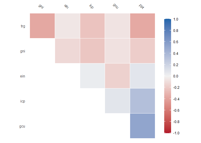
We can calculate and visualise correlations:

#In built xgboost imputation function
mdl$correlate()
#> Key: 
#>   key                             indicator
#> 1 ein Energy imports, net (% of energy use)
#> 2 gcu                     GDP (current US$)
#> 3 gni                            Gini index
#> 4 icp Inflation, consumer prices (annual %)
#> 5 ppt                     Population, total
#> 6 trg                      Trade (% of GDP)
#> Correlation computed with
#> • Method: 'pearson'
#> • Missing treated using: 'pairwise.complete.obs'

#> # A tibble: 6 × 7
#>   term      ein     gcu     gni     icp     ppt     trg
#>   <chr>   <dbl>   <dbl>   <dbl>   <dbl>   <dbl>   <dbl>
#> 1 ein   NA      -0.161  -0.123   0.0364  0.0805 -0.0568
#> 2 gcu   -0.161  NA      -0.0786  0.0810  0.526  -0.0676
#> 3 gni   -0.123  -0.0786 NA      -0.216  -0.178  -0.367 
#> 4 icp    0.0364  0.0810 -0.216  NA       0.341  -0.231 
#> 5 ppt    0.0805  0.526  -0.178   0.341  NA      -0.364 
#> 6 trg   -0.0568 -0.0676 -0.367  -0.231  -0.364  NA

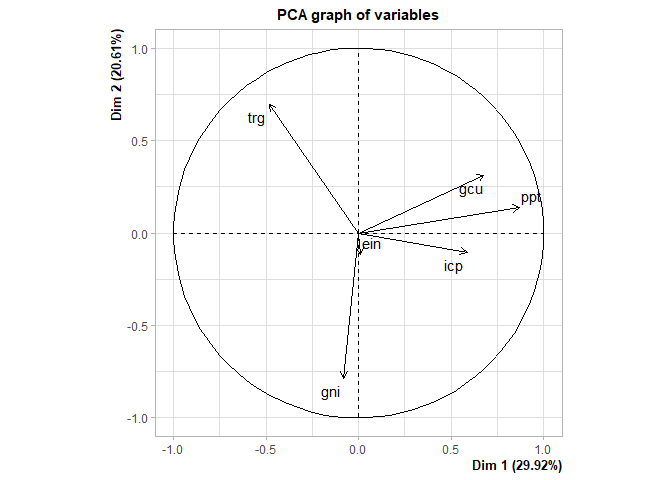
We can also perform principal component analysis:

# In built principal components analysis function
tmp <- mdl$pca()
#> Warning in PCA(self$child, graph = FALSE): Missing values are imputed by the
#> mean of the variable: you should use the imputePCA function of the missMDA
#> package
plot(tmp, choix = "var")

We can also append any data to the original data frame so long as the newdata is either:

• A vector where length(newdata) = nrow(mdl$child)
• A marix/dataframe where identical(dim(newdata), dim(mdl$child)) == TRUE

### Can be used to add a yhat value for processed data

nc <- ncol(mdl$child)
nr <- nrow(mdl$child)
dm <- nc * nr
dummy <- matrix(runif(dm),
                ncol = nc) |>
                data.frame()
names(dummy) = names(mdl$child)
tmp <- mdl$assemble(dummy)
head(tmp)
#> # A tibble: 6 × 5
#>   iso3c indicator                              year    value  yhat
#>   <chr> <chr>                                 <dbl>    <dbl> <dbl>
#> 1 DZA   Energy imports, net (% of energy use)  2012 -2.13e 2 0.541
#> 2 DZA   GDP (current US$)                      2012  2.27e11 0.220
#> 3 DZA   Gini index                             2012 NA       0.952
#> 4 DZA   Inflation, consumer prices (annual %)  2012  8.89e 0 0.638
#> 5 DZA   Population, total                      2012  3.73e 7 0.382
#> 6 DZA   Trade (% of GDP)                       2012  6.08e 1 0.223
### This is useful for imputation purposes as below