Identifying Important Areas from Animal Tracking Data.
track2KBA 
This package is comprised of functions that facilitate the identification of areas of importance for biodiversity, such as Key Biodiversity Areas (KBAs), based on individual tracking data. For further detail concerning the method itself, please refer to this paper by Beal et al. (2021).
Key functions include utilities to estimate individual core use areas, the level of representativeness of the tracked sample, and overlay individual distributions to identify important sites at the population level. Other functions assist in plotting the results, formatting your data set, and splitting and summarizing individual foraging trips.
Installation
You can download the stable version from CRAN with:
install.packages("track2KBA")
Or you can download the development version from GitHub with:
install.packages("devtools", dependencies = TRUE)
devtools::install_github("BirdLifeInternational/track2kba", dependencies=TRUE) # development version - add argument 'build_vignettes = FALSE' to speed it up
Example
Now we will use tracking data collected at a seabird breeding colony to illustrate a track2KBA workflow for identifying important sites. It is important to note that the specific workflow you use (i.e., which functions and in what order) will depend on the species of interest and the associated data at hand.
First, in order for the data to work in track2KBA functions, we can use the formatFields function to format the important data columns needed for analysis. These are: a DateTime field, Latitude and Longitude fields, and an ID field (i.e. individual animal, track, or trip).
library(track2KBA) # load package

data(boobies)
# ?boobies  # for some background info on the example data set

dataGroup <- formatFields(
  dataGroup = boobies,
  fieldID   = "track_id",
  fieldDate = "date_gmt",
  fieldTime = "time_gmt",
  fieldLon  = "longitude",
  fieldLat  = "latitude"
  )

str(dataGroup)
If your data come from a central-place foraging species (i.e. one which makes trips out from a centrally-located place, such as a nest in the case of a bird), you can use tripSplit to split up the data into discrete trips.
In order to do this, you must identify the location(s) of the central place(s) (e.g. colony-center, or nest sites).
library(dplyr)

# here we know that the first points in the data set are from the colony center
colony <- dataGroup %>%
  summarise(
    Longitude = first(Longitude),
    Latitude  = first(Latitude)
    )
Our colony dataframe tells us where trips originate from. Then we can set some parameters to decide what constitutes a trip. To do that we should use our understanding of the movement ecology of the study species. In this case we know our seabird travels out to sea on the scale of tens of kilometers, so we set innerBuff (the minimum distance from the colony) to 3 km, and duration (minimum trip duration) to 1 hour. returnBuff can be set further out in order to catch incomplete trips, where the animal began returning, but perhaps due to device failure the full trip wasn’t captured.
Optionally, we can set rmNonTrip to TRUE which will remove the periods when the animals were not on trips. The results of tripSplit can be plotted using mapTrips to see some examples of trips.
str(dataGroup)

trips <- tripSplit(
  dataGroup  = dataGroup,
  colony     = colony,
  innerBuff  = 3,      # kilometers
  returnBuff = 10,
  duration   = 1,      # hours
  rmNonTrip  = TRUE
  )

mapTrips(trips = trips, colony = colony)
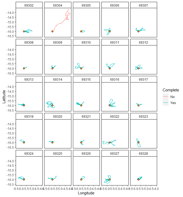
Then we can summarize the trip movements, using tripSummary. First, we can filter out data from trips that did not return to the vicinity of the colony (i.e. within returnBuff), so they don’t skew the estimates.
trips <- subset(trips, trips$Returns == "Yes" )

sumTrips <- tripSummary(trips = trips, colony = colony)

sumTrips
Now that we have an idea how the animals are moving, we can start with the process of estimating their space use areas, and identifying potentially important sites for the population!
track2KBA uses Kernel Density Estimation (KDE) to produce space use estimates for each individual track. In order for these to be accurate, we need to transform the tracking data to an equal-area projection. We can use the convenience function projectTracks to perform this projection. We can select between an azimuthal or cylindrical projection, and decide whether to center the projection on the data itself. Custom-centering is generally a good idea for quick analyses as this will minimize distortion, however it is important to remember that the resulting projection will be data specific. So if you remove even one track and re-analyze, the projection will differ between datasets. For formal analysis, the best solution is to find a standard projection that is appropriate for your study region.
tracks <- projectTracks( dataGroup = trips, projType = 'azim', custom=TRUE )
class(tracks)
findScale provides options for setting the all-important smoothing parameter in the KDE. This parameter decisions is of the utmost importance, as it determines the scale at which the tracking locations will be ‘smoothed’ into an estimate of the probability of use of space by the animal. findScale calculates candidate smoothing parameter values using several different methods.
If we know our animal uses an area-restricted search (ARS) strategy to locate prey, then we can set the scaleARS=TRUE. This uses First Passage Time analysis to identify the spatial scale at which area-restricted search is occuring, which may then be used as the smoothing parameter value.
hVals <- findScale(
  tracks   = tracks,
  scaleARS = TRUE,
  sumTrips = sumTrips)

hVals
The other values provided by findScale are more simplistic methods of calculating the smoothing parameter. href is the canonical reference method, and relates to the number of points in the data and their spatial variance. mag is the log of the average foraging range (med_max_dist in the sumTrips output); this methods only works for central-place foragers.
Next, we must select a smoothing parameter value. To inform our decision, we ought to use our understanding of the species’ movement ecology to guide our decision about what scale make sense. That is, from the findScale output, we want to avoid using values which may under- or over-represent the area used by the animals while foraging.
Once we have chosen a smoothing value, we can produce KDEs for each individual, using estSpaceUse. By default this function isolates the core range of each track (i.e. the 50% utilization distribution, or where the animal spends about half of its time) which is a commonly used standard (Lascelles et al. 2016). However, another quantile can be chose using the levelUD argument, or the full utilization distritbution can be returned using polyOut=FALSE.
The resulting KDEs can be plotted using mapKDE, which if polyOut=TRUE shows each tracks’s core range in a different color.
Note: here we might want to remove the trip start and end points that fall within the innerBuff (i.e. 3 km) we set in tripSplit, so that they don’t skew the at-sea distribution towards to colony.
tracks <- tracks[tracks$ColDist > 3, ] # remove trip start and end points near colony

KDE <- estSpaceUse(
  tracks = tracks,
  scale = hVals$mag,
  levelUD = 50,
  polyOut = TRUE
  )

mapKDE(KDE = KDE$UDPolygons, colony = colony)
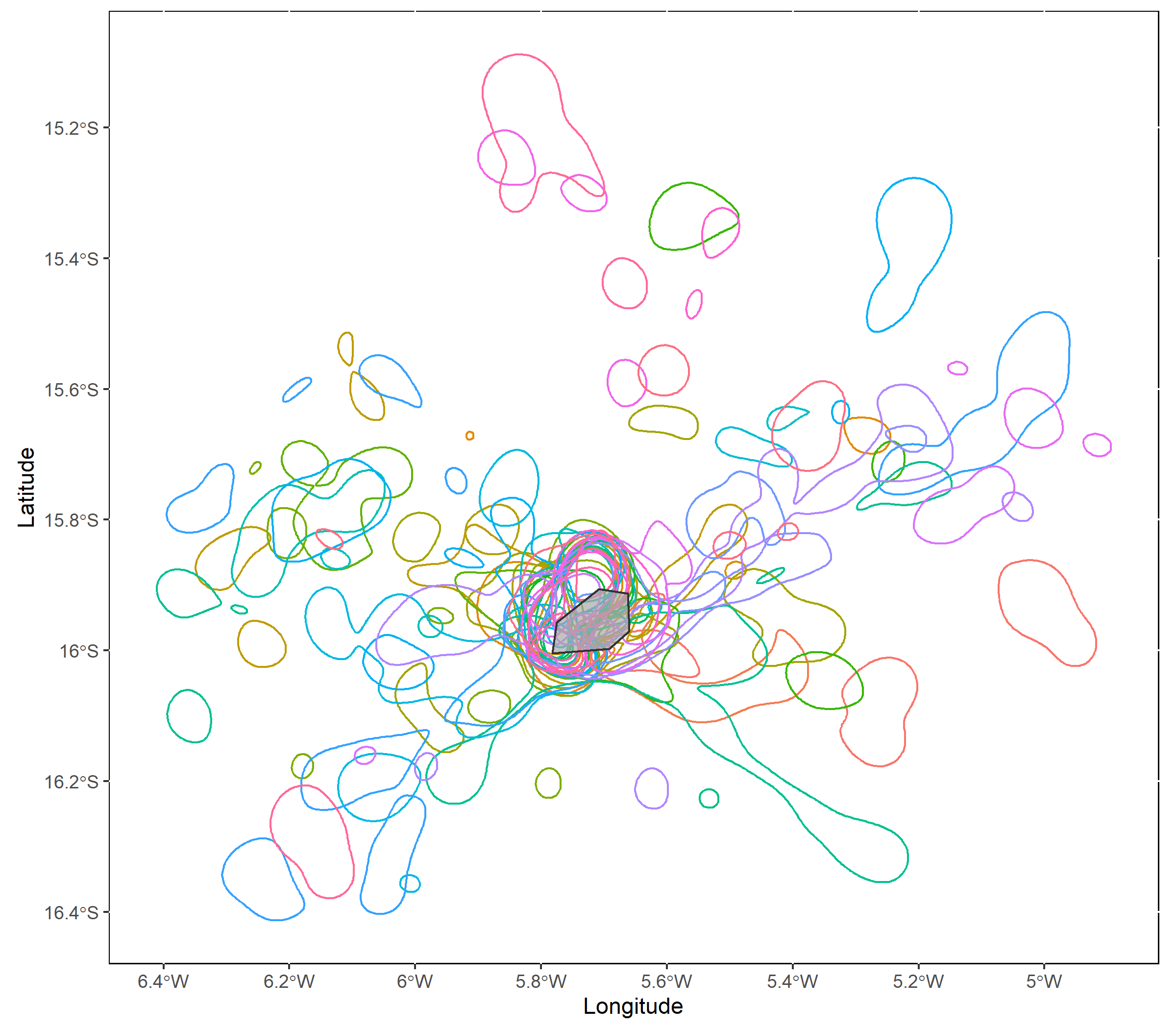 At this step we should verify that the smoothing parameter value we selected is producing reasonable space use estimates, given what we know about our study animals. Are the core areas much larger than expected? Much smaller? If so, consider using a different value for the `scale` parameter.
 The next step is to estimate how representative this sample of animals is of the population. That is, how well does the variation in space use of this sample of tracks encapsulate variation in the wider population? To do this we can use the repAssess function. This function repeatedly samples a subset of track core ranges, averages them together, and quantifies how many points from the unselected tracks fall within this combined core range area. This process is run across the range of the sample size, and iterated a chosen number of times.
To do this, we need to supply Utilization Distributions to repAssess (e.g., the output of estSpaceUse) and the tracking data. We can choose the number of times we want to re-sample at each sample size by setting the iteration argument. The higher the number the more confident we can be in the results, but the longer it will take to compute.
repr <- repAssess(
  tracks    = tracks,
  KDE       = KDE$KDE.Surface,
  levelUD   = 50,
  iteration = 1,
  bootTable = FALSE)
The output is a dataframe, with the estimated percentage of representativeness given in the out column.
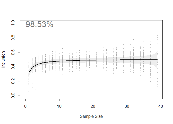
The relationship between sample size and the percent coverage of un-tested animals’ space use areas (i.e. Inclusion) is visualized in the output plot seen below.
By quantifying this relationship, we can estimate how close we are to an information asymptote. Put another way, we have estimated how much new space use information would be added by tracking more animals. In the case of this seabird dataset, we estimate that ~98% of the core areas used by this population are captured by the sample of 39 individuals. Highly representative!
Now, using findSite we can identify areas where animals are overlapping in space and delineate sites that meet some criteria of importance. Using the core area estimates of each individual track we can calculate where they overlap. Then, we estimate the proportion of the larger population in a given area by adjusting our overlap estimate based on the degree of representativeness.
Here, if we have population size estimates, we can include this value (using the popSize argument) to estimate the number of individuals using a space, which can then use to compare against population-level importance criteria (e.g. KBA criteria). If we don’t have population size estimates to provide, findSite this will output a proportion of the population instead.
If you desire polygon output of the overlap areas, instead of a gridded surface, you can indicate this using the polyOut argument.
Site <- findSite(
  KDE = KDE$KDE.Surface,
  represent = repr$out,
  levelUD = 50,
  popSize = 500,     # 500 individual seabirds breed one the island
  polyOut = TRUE
  )

class(Site)
If we specified polyOut=TRUE, then the output will be of Simple Features class, which allows us to easily take advantage of the ggplot2 plotting syntax to make an attractive map using mapSite!
Sitemap <- mapSite(Site, colony = colony)
## in case you want to save the plot
# ggplot2::ggsave("KBAmap", device="png")
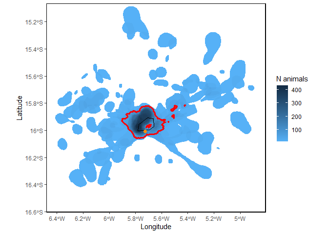
This map shows the number or proportion of individual animals in the population overlapping in space. The red lines indicate the ‘potential site’; that is, the areas used by a significant proportion of the local population, given the representativeness of the sample of tracked individuals. In this case, since representativeness is >90%, any area used by 10% or more of the population is considered important (see Lascelles et al. 2016 for details). The orange dot is the colony location and the black line is the coastline.
Note: it is possible to set the threshold of importance at the population level yourself, using the thresh argument. Just be aware that this is a crucial threshold parameter that will need justifying if you are to eventually recommend a site for formal acknowledgement as an important site for conservation.
Then, we can combine all the polygons within the ‘potentialSite’ area, and use, for example, the maximum number of individuals present in that area to assess whether it may merits identification as a Key Biodiversity Area according to the KBA standard.
potSite <- Site %>% dplyr::filter(.data$potentialSite==TRUE) %>%
   summarise(
     max_animals = max(na.omit(N_animals)), # maximum number of animals aggregating in the site
     min_animals = min(na.omit(N_animals))  # minimum number using the site
   )
If in findSite we instead specify polyOut=FALSE, our output will be a spatial grid of animal densities, with each cell representing the estimated number, or percentage of animals using that area. So this output is independent of the representativness-based importance threshold.
mapSite(Site, colony = colony)
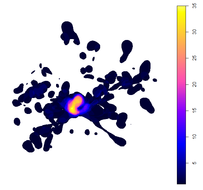
This plot shows the minimum estimated number of birds using the space around the breeding island.
Package reference
If you use any functions in this package for your work, please use the following citation:
Beal, M., Oppel, S., Handley, J., Pearmain, E. J., Morera-Pujol, V., Carneiro, A. P. B., Davies, T. E., Phillips, R. A., Taylor, P. R., Miller, M. G. R., Franco, A. M. A., Catry, I., Patrício, A. R., Regalla, A., Staniland, I., Boyd, C., Catry, P., & Dias, M. P. (2021). track2KBA: An R package for identifying important sites for biodiversity from tracking data. Methods in Ecology and Evolution, 12(12), 2372-2378. https://doi.org/10.1111/2041-210X.13713
Example data reference
Oppel, S., Beard, A., Fox, D., Mackley, E., Leat, E., Henry, L., Clingham, E., Fowler, N., Sim, J., Sommerfeld, J., Weber, N., Weber, S., Bolton, M., 2015. Foraging distribution of a tropical seabird supports Ashmole’s hypothesis of population regulation. Behav Ecol Sociobiol 69, 915–926. https://doi.org/10.1007/s00265-015-1903-3
Other references
Lascelles, B. G., Taylor, P. R., Miller, M. G. R., Dias, M. P., Oppel, S., Torres, L., Hedd, A., Corre, M. L., Phillips, R. A., Shaffer, S. A., Weimerskirch, H., & Small, C. (2016). Applying global criteria to tracking data to define important areas for marine conservation. Diversity and Distributions, 22(4), 422–431. https://doi.org/10.1111/ddi.12411
Acknowledgements
Thanks to Annalea Beard for kindly sharing these example data for use in the package.
This project has received funding from the European Union’s Horizon 2020 research and innovation programme under the Marie Skłodowska-Curie grant agreement No 766417.