Colorblind-Friendly Palettes from Washington State.
Colorblind-friendly Palettes from Washington State
The wacolor package contains 28 color palettes taken from the landscapes and cities of Washington state. Colors were extracted from a set of photographs, and then combined to form a set of continuous and discrete palettes. Continuous palettes were designed to be perceptually uniform, while discrete palettes were chosen to maximize contrast at several different levels of overall brightness and saturation. Each palette has been evaluated to ensure colors are distinguishable by colorblind people.
Discrete palettes contain at most seven colors. Don’t create graphics that use more than seven discrete colors. You can color a map with four. Anything more risks confusion. Consider differentiating through faceting or labels, instead.
Installation
You can install the released version of wacolors from CRAN with:
install.packages("wacolors")
You can install the development version of wacolors from GitHub with:
devtools::install_github("CoryMcCartan/wacolors")
Usage
It’s easy to select a palette. Access palettes through wacolors$... for autocompletion suggestions.
library(wacolors)
library(ggplot2)

# See all palettes
names(wacolors)
#>  [1] "rainier"         "washington_pass" "palouse"         "forest"
#>  [5] "larch"           "coast"           "san_juan"        "uw"
#>  [9] "fort_worden"     "skagit"          "flag"            "sound_sunset"
#> [13] "ferries"         "forest_fire"     "sea"             "sea_star"
#> [17] "volcano"         "baker"           "diablo"          "puget"
#> [21] "mountains"       "gorge"           "foothills"       "footbridge"
#> [25] "olympic"         "lopez"           "vantage"         "stuart"

# See one palette
wacolors$rainier
#>       lake    ragwort      lodge      trees     ground winter_sky paintbrush
#>  "#465177"  "#E4C22B"  "#965127"  "#29483A"  "#759C44"  "#9FB6DA"  "#DF3383"
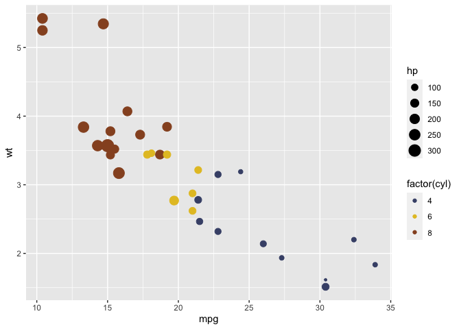
The package comes with ggplot2-compatible scales which are easy to use.
# access by name
ggplot(mtcars, aes(mpg, wt)) +
    geom_point(aes(color = factor(cyl), size=hp)) +
    scale_color_wa_d("rainier")

# or access using `wacolors$...`
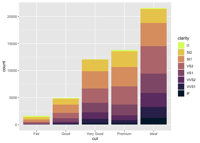
ggplot(diamonds) +
    geom_bar(aes(x = cut, fill = clarity)) +
    scale_fill_wa_d(wacolors$sound_sunset, reverse=TRUE)

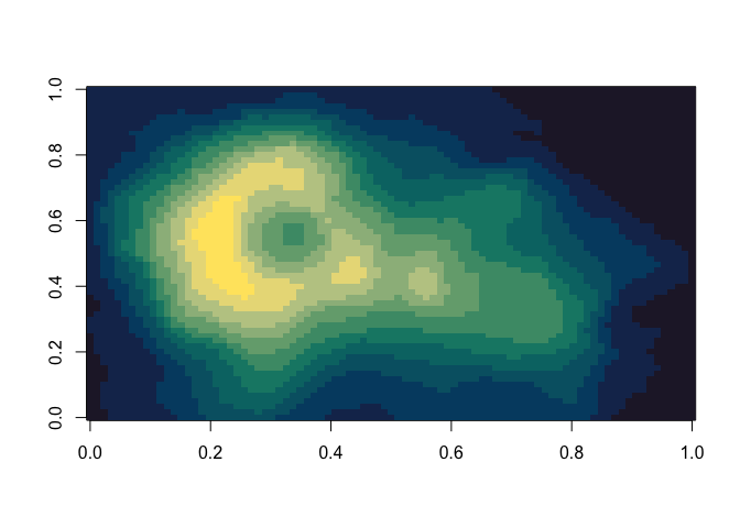
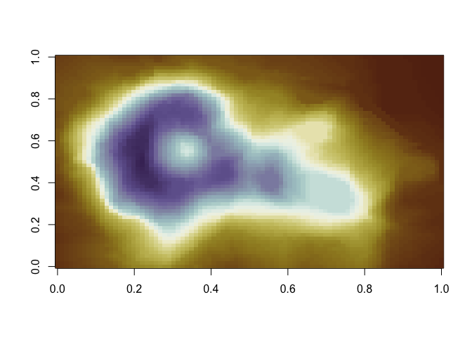
You can use the wa_pal function to directly construct a discretized/binned color scale.
image(volcano, col=wa_pal("ferries", 12))

image(volcano, col=wa_pal("vantage", 200, reverse=TRUE))

Code Generation
In case you do not wish to have wacolors as a dependency, you may use the pal_vector() and pal_functions() functions, which generate self-contained code for using the palettes. When using RStudio, this code will be loaded, ready to copy, at the console prompt.
pal_vector("sound_sunset", 15)
#> PAL_SOUND_SUNSET = c("#001E35", "#0E2648", "#342C59", "#523368", "#6D3D71",
#>                      "#804C73", "#925B78", "#A16C7B", "#BB797D", "#D08B79",
#>                      "#DE9F71", "#E6B465", "#EBCC5B", "#E6E55B", "#DCFF6C")

pal_functions("palouse")
#> scale_color_palouse_d = function(...) {
#>   pal_cols = c("#2D3F4A", "#C0A43D", "#8A6172", "#748A52", "#CCBA98",
#>                "#69A2E4")
#>   n_col = length(pal_cols)
#>   ramp = grDevices::colorRampPalette(pal_cols)
#>   pal_fun = function(n) if (n <= n_col) pal_cols[1:n] else ramp(n)
#>   discrete_scale("color", "palouse", palette=pal_fun, ...)
#> }
#> scale_fill_palouse_d = function(...) {
#>   pal_cols = c("#2D3F4A", "#C0A43D", "#8A6172", "#748A52", "#CCBA98",
#>                "#69A2E4")
#>   n_col = length(pal_cols)
#>   ramp = grDevices::colorRampPalette(pal_cols)
#>   pal_fun = function(n) if (n <= n_col) pal_cols[1:n] else ramp(n)
#>   discrete_scale("fill", "palouse", palette=pal_fun, ...)
#> }
#>
#> scale_color_palouse_c = function(...) {
#>   scale_color_gradientn(..., colours=c("#2D3F4A", "#C0A43D", "#8A6172",
#>                         "#748A52", "#CCBA98", "#69A2E4"))
#> }
#> scale_fill_palouse_c = function(...) {
#>   scale_fill_gradientn(..., colours=c("#2D3F4A", "#C0A43D", "#8A6172",
#>                        "#748A52", "#CCBA98", "#69A2E4"))
#> }
#>
#>
The Palettes
Continuous Palettes


Discrete Palettes.


