Statistical Methods for Life Data Analysis.

weibulltools

Overview

The {weibulltools} package focuses on statistical methods and visualizations that are often used in reliability engineering. It provides a compact and easily accessible set of methods and visualization tools that make the examination and adjustment as well as the analysis and interpretation of field data (and bench tests) as simple as possible.

Besides the well-known Weibull analysis, the package supports multiple lifetime distributions and also contains Monte Carlo methods for the correction and completion of imprecisely recorded or unknown lifetime characteristics.

Plots are created statically {ggplot2} or interactively {plotly} and can be customized with functions of the respective visualization package.

Installation

The latest released version of {weibulltools} from CRAN can be installed with:

install.packages("weibulltools")

Development version

Install the development version of {weibulltools} from GitHub to use new features or to get a bug fix.

# install.packages("devtools")
devtools::install_github("Tim-TU/weibulltools")

Usage

Getting started

Create consistent reliability data with columns:

• x - lifetime characteristic
• status - binary data (0 for censored units and 1 for failed units)
• id (optional) - identifier for units

library(weibulltools)

rel_tbl <- reliability_data(data = shock, x = distance, status = status)
rel_tbl
#> Reliability Data with characteristic x: 'distance':
#> # A tibble: 38 × 3
#>       x status id   
#>   <int>  <dbl> <chr>
#> 1  6700      1 ID1  
#> 2  6950      0 ID2  
#> 3  7820      0 ID3  
#> 4  8790      0 ID4  
#> 5  9120      1 ID5  
#> # … with 33 more rows

Probability estimation and visualization

Estimation of failure probabilities using different non-parametric methods:

prob_tbl <- estimate_cdf(x = rel_tbl, methods = c("mr", "kaplan", "johnson", "nelson"))
#> The 'mr' method only considers failed units (status == 1) and does not retain intact units (status == 0).
prob_tbl
#> CDF estimation for methods 'mr', 'kaplan', 'johnson', 'nelson':
#> # A tibble: 125 × 6
#>   id        x status  rank   prob cdf_estimation_method
#>   <chr> <int>  <dbl> <dbl>  <dbl> <chr>                
#> 1 ID1    6700      1     1 0.0614 mr                   
#> 2 ID5    9120      1     2 0.149  mr                   
#> 3 ID13  12200      1     3 0.237  mr                   
#> 4 ID15  13150      1     4 0.325  mr                   
#> 5 ID19  14300      1     5 0.412  mr                   
#> # … with 120 more rows

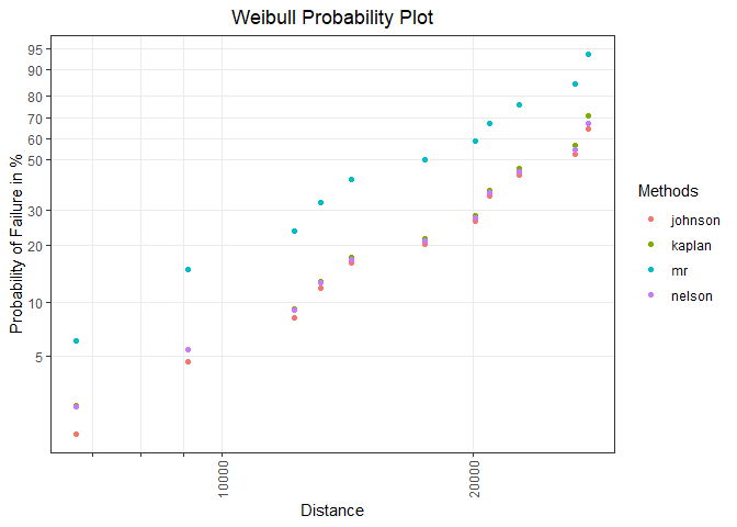
Visualization of the obtained results in a distribution-specific probability plot:

prob_vis <- plot_prob(x = prob_tbl, distribution = "weibull", 
                      title_main = "Weibull Probability Plot", 
                      title_x = "Distance", 
                      title_y = "Probability of Failure in %", 
                      title_trace = "Methods",
                      plot_method = "gg")
prob_vis

Model estimation and visualization

Parametric model estimation with respect to the used methods:

rr_list <- rank_regression(x = prob_tbl, distribution = "weibull")
rr_list
#> List of 4 model estimations:
#> Rank Regression
#> Coefficients:
#>      mu    sigma  
#> 10.2596   0.3632  
#> Method of CDF Estimation: johnson 
#> 
#> Rank Regression
#> Coefficients:
#>      mu    sigma  
#> 10.2333   0.3773  
#> Method of CDF Estimation: kaplan 
#> 
#> Rank Regression
#> Coefficients:
#>     mu   sigma  
#> 9.8859  0.3956  
#> Method of CDF Estimation: mr 
#> 
#> Rank Regression
#> Coefficients:
#>      mu    sigma  
#> 10.2585   0.3852  
#> Method of CDF Estimation: nelson

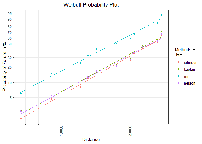
Model visualization in an existing probability plot:

mod_vis <- plot_mod(p_obj = prob_vis, x = rr_list, distribution = "weibull", 
                    title_trace = "RR") 
mod_vis

Getting help

If you notice a bug or have suggestions for improvements, please submit an issue with a minimal reproducible example on GitHub. For further questions, please contact Tim-Gunnar Hensel.