White Test and Bootstrapped White Test for Heteroskedasticity.
whitestrap
This package presents the White’s Test of Heterocedasticity and a bootstrapped version of it, developed under the methodology of Jeong, J., Lee, K. (1999) (see references for further details).
Installation
You can install the development version from GitHub with:
# install.packages("devtools")
devtools::install_github("jlopezper/whitestrap")
Example
This is an example which shows you how you can use the white_test and white_test_boot functions:
library(whitestrap)
#>
#> Please cite as:
#> Lopez, J. (2020), White's test and Bootstrapped White's test under the methodology of Jeong, J., Lee, K. (1999) package version 0.0.1

set.seed(123)
# Let's simulate some heteroscedastic data
n <- 100
y <- 1:n
sd <- runif(n, min = 0, max = 4)
error <- rnorm(n, 0, sd*y)
X <- y + error
df <- data.frame(y, X)
# OLS model
fit <- lm(y ~ X, data = df)
# White's test and Bootstrapped White's test
white_test(fit)
#> White's test results
#>
#> Null hypothesis: Homoskedasticity of the residuals
#> Alternative hypothesis: Heteroskedasticity of the residuals
#> Test Statistic: 12.88
#> P-value: 0.001597
white_test_boot(fit)
#> Bootstrapped White's test results
#>
#> Null hypothesis: Homoskedasticity of the residuals
#> Alternative hypothesis: Heteroskedasticity of the residuals
#> Number of bootstrap samples: 1000
#> Boostrapped Test Statistic: 12.88
#> P-value: 0.003
In either case, the returned object is a list with the value of the statistical test and the p-value of the test. For the bootstrapped version, the number of bootstrap samples is also provided.
names(white_test(fit))
#> [1] "w_stat"  "p_value"
names(white_test_boot(fit))
#> [1] "w_stat"  "p_value" "iters"
Comparison between the original and the bootstrap version
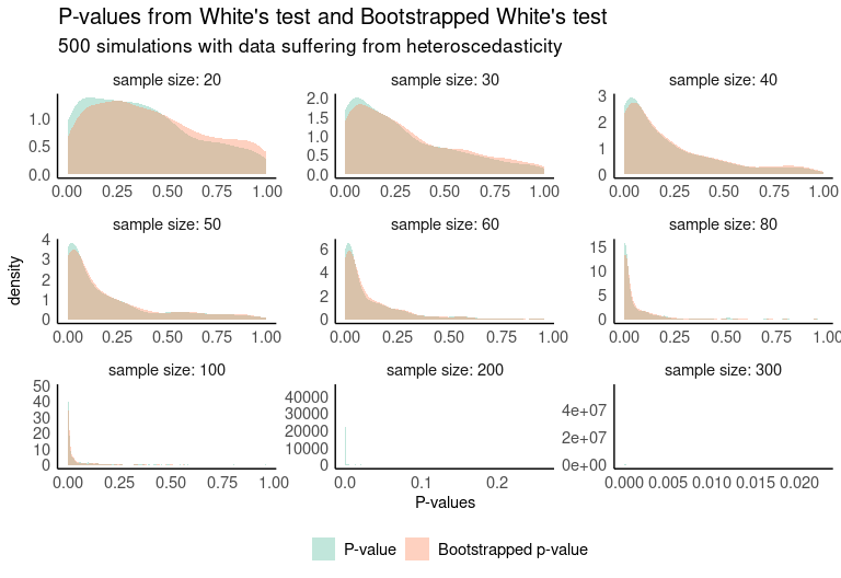
One way to compare the results of both tests is through simulations. The following plot shows the distribution of 500 simulations where the p-value of both tests is computed. The data used for this purpose were artificially generated to be heterocedastic, so low p-values are desirable.

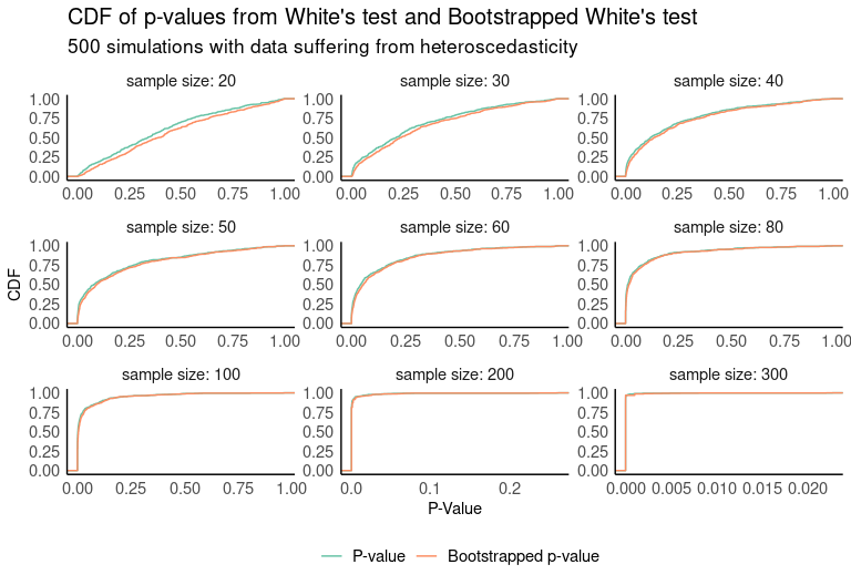
If we look at the cumulative distribution functions of both p-value distributions, we see that in small samples the bootstrapped test returns smaller p-values with higher probability.

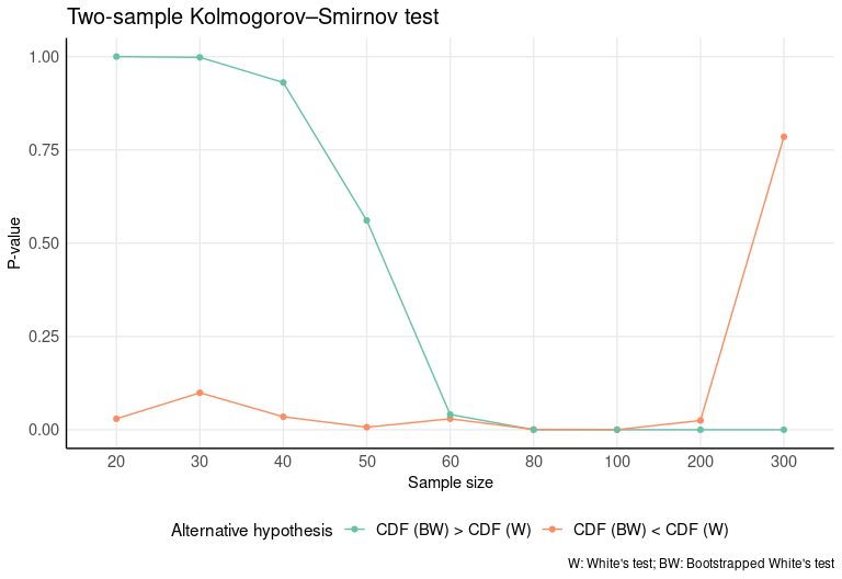
In order to check for differences between the two distributions, a two-sample Kolmogorov–Smirnov test is run. In this case, we’ll test whether one distribution stochastically dominates another, so the test will be run for both alternative sides (CDF (BW) > CDF (W) and CDF (BW) < CDF (W)). We see from the results that CDF (BW) statistically outperforms CDF (W) for samples < 60. No differences are appreciated with samples greater than or equal to 60.

References
Jeong, J., & Lee, K. (1999). Bootstrapped White’s test for heteroskedasticity in regression models. Economics Letters, 63(3), 261-267.
White, H. (1980). A Heteroskedasticity-Consistent Covariance Matrix Estimator and a Direct Test for Heteroskedasticity. Econometrica, 48(4), 817-838.
Wooldridge, Jeffrey M., 1960-. (2012). Introductory econometrics : a modern approach. Mason, Ohio, South-Western Cengage Learning.
